MLflow Tutorial for Machine Learning in Python — Part 3: Log Artifacts and Datasets

Part 2's runs record numbers: scores at every step and the computer's load. Two questions those numbers can't answer: which data did this run learn from, and what did it produce besides scores? In this part every run records its training, validation and test data as MLflow datasets, and saves three files with itself: which features the forest relies on, every setting it used, and every prediction it got wrong.
This is Part 3 of a 10-part series.
- Part 1: Install MLflow and Track Your First Experiment
- Part 2: Log Metrics Over Time and System Metrics
- Part 3: Log Artifacts and Datasets (you are here)
- Part 4: Search and Filter Runs (coming soon)
- Part 5: Autologging and Hyperparameter Tuning with Nested Runs (coming soon)
- Part 6: Log, Load and Validate Models (coming soon)
- Part 7: Evaluate Models and Set Quality Gates (coming soon)
- Part 8: Register, Version and Promote Models with the Model Registry (coming soon)
- Part 9: Serve a Model as a REST API and in Docker (coming soon)
- Part 10: Production Checklist and Recap (coming soon)
Every command and output on this page is real, captured while building the project.
What You'll Build in This Part
You'll keep working on the house price project and add:
- datasets: each run records the three parts of the data it used, training, validation and test, with a fingerprint of their contents (the digest), their source, their columns and their size;
- a feature importance table, logged with
mlflow.log_table(), which the UI can show for several runs side by side; - the forest's complete settings, logged as a JSON file with
mlflow.log_dict(); - a CSV file of every test prediction and its error, biggest misses first, logged with
mlflow.log_artifact(); - comparisons in the MLflow UI: which runs used the same data, and how their files differ.
Two words for this part. An artifact is any file stored with a run, such as Part 1's chart. A dataset, in MLflow, is a record of the data a run used, not the data itself.
What This Part Costs
Nothing. Everything runs on your own computer, and there are no new packages.
Prerequisites
- Part 2 finished: the
mlflow-serverfolder with its runs, and thedewiride-house-price-predictionproject, committed to Git. Part 2 builds on Part 1 for both.
Step 1: Start the Tracking Server
Open a terminal in the mlflow-server folder and start the server, as before:
uv run mlflow server --port 8080
Wait for Application startup complete, leave it running, and open a second terminal in the dewiride-house-price-prediction folder for everything else.
Step 2: Note Where the Data Comes From
A dataset record includes its source: where the data came from, so anyone can find the original later. scikit-learn's fetch_california_housing() downloads the California Housing data from one fixed address, so that address is the source. Open src/house_price_prediction/data.py and add it below TARGET:
TARGET = "MedHouseVal"
# The file scikit-learn downloads the California Housing data from.
SOURCE_URL = "https://ndownloader.figshare.com/files/5976036"
The complete file:
"""Load the California Housing data and split it for training, validation and testing."""

from dataclasses import dataclass

import pandas as pd
from sklearn.datasets import fetch_california_housing
from sklearn.model_selection import train_test_split

TARGET = "MedHouseVal"
# The file scikit-learn downloads the California Housing data from.
SOURCE_URL = "https://ndownloader.figshare.com/files/5976036"


@dataclass(frozen=True)
class DataSplit:
    """The features and target values for training, validation and testing."""

    X_train: pd.DataFrame
    X_val: pd.DataFrame
    X_test: pd.DataFrame
    y_train: pd.Series
    y_val: pd.Series
    y_test: pd.Series


def load_housing_data() -> pd.DataFrame:
    """Return the dataset as one table. The first call downloads it; later calls read a cache."""
    return fetch_california_housing(as_frame=True).frame


def split_data(
    frame: pd.DataFrame, test_size: float, validation_size: float, random_state: int
) -> DataSplit:
    """Hold back `test_size` of the rows for the final test, then `validation_size` of the rest
    to watch the model while it trains. The model learns from what is left."""
    features = frame.drop(columns=TARGET)
    target = frame[TARGET]
    X_rest, X_test, y_rest, y_test = train_test_split(
        features, target, test_size=test_size, random_state=random_state
    )
    X_train, X_val, y_train, y_val = train_test_split(
        X_rest, y_rest, test_size=validation_size, random_state=random_state
    )
    return DataSplit(X_train, X_val, X_test, y_train, y_val, y_test)
Step 3: Describe Each Part of the Split as a Dataset
mlflow.data.from_pandas() turns a pandas table into an MLflow dataset. It computes three things from the table, without storing the table itself:
- a digest, an 8-character fingerprint of the contents: the same data gives the same digest in every run;
- a schema, each column with its type;
- a profile, the number of rows and of values.
The split keeps each part's features and target values apart, in X_train and y_train and so on. A dataset should hold both, with the target marked, so each part is joined back into one table first. Create src/house_price_prediction/datasets.py:
"""Describe the data each run trains, validates and tests on, so MLflow can record it."""

import mlflow.data
import pandas as pd
from mlflow.data.pandas_dataset import PandasDataset

from house_price_prediction.data import SOURCE_URL, TARGET, DataSplit


def as_dataset(features: pd.DataFrame, target: pd.Series, name: str) -> PandasDataset:
    """One part of the split as an MLflow dataset: its features with the target column added."""
    return mlflow.data.from_pandas(
        features.join(target), source=SOURCE_URL, targets=TARGET, name=name
    )


def split_datasets(data: DataSplit) -> dict[str, PandasDataset]:
    """The three parts of the split, each under the context MLflow records it with."""
    return {
        "training": as_dataset(data.X_train, data.y_train, "california-housing-train"),
        "validation": as_dataset(data.X_val, data.y_val, "california-housing-validation"),
        "testing": as_dataset(data.X_test, data.y_test, "california-housing-test"),
    }
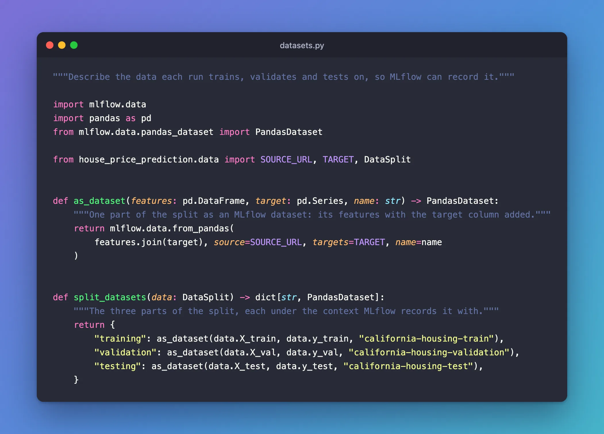
features.join(target)adds the target column to the features, matching rows by their labels: How to Join a pandas Series to a DataFrame by Index.source=SOURCE_URLrecords the download address. Because it starts withhttps://, MLflow stores it as a web source, and the UI offers to open it.targets=TARGETmarksMedHouseValas the column the model predicts.name=gives each part a readable name; without it, every dataset would be calleddataset.- The dictionary's keys,
training,validationandtesting, are the contexts: what the run used each part for. They're the labels MLflow's own examples use.
Step 4: Log the Datasets with Each Run
mlflow.log_input() attaches a dataset to the active run, with its context. In src/house_price_prediction/train.py, import the new module:
from house_price_prediction.datasets import split_datasets
Then log the three datasets right after the run's tags, before training starts:
        mlflow.set_tags({"model_type": "random_forest", "dataset": "california_housing"})
        for context, dataset in split_datasets(data).items():
            mlflow.log_input(dataset, context=context)
Three calls, one per part. Only the description travels to the tracking server; the data stays on your computer.
Step 5: Turn the Trained Forest into Two Tables
Two tables are worth keeping with every run: which inputs the forest relies on, and where its predictions go wrong. Create src/house_price_prediction/reports.py:
"""Tables that show what the trained model relies on and where it goes wrong."""

import numpy as np
import pandas as pd
from sklearn.ensemble import RandomForestRegressor


def feature_importances(model: RandomForestRegressor) -> pd.DataFrame:
    """How much each feature helped the forest's splits, most important first."""
    table = pd.DataFrame(
        {"feature": model.feature_names_in_, "importance": model.feature_importances_}
    )
    return table.sort_values("importance", ascending=False, ignore_index=True)


def prediction_errors(
    X_test: pd.DataFrame, y_test: pd.Series, predictions: np.ndarray
) -> pd.DataFrame:
    """Every test row's true value, the model's prediction and its error, then the row's
    features. The biggest errors come first."""
    table = pd.DataFrame(
        {y_test.name: y_test, "Prediction": predictions, "Error": predictions - y_test}
    ).join(X_test)
    return table.sort_values("Error", key=abs, ascending=False, ignore_index=True)
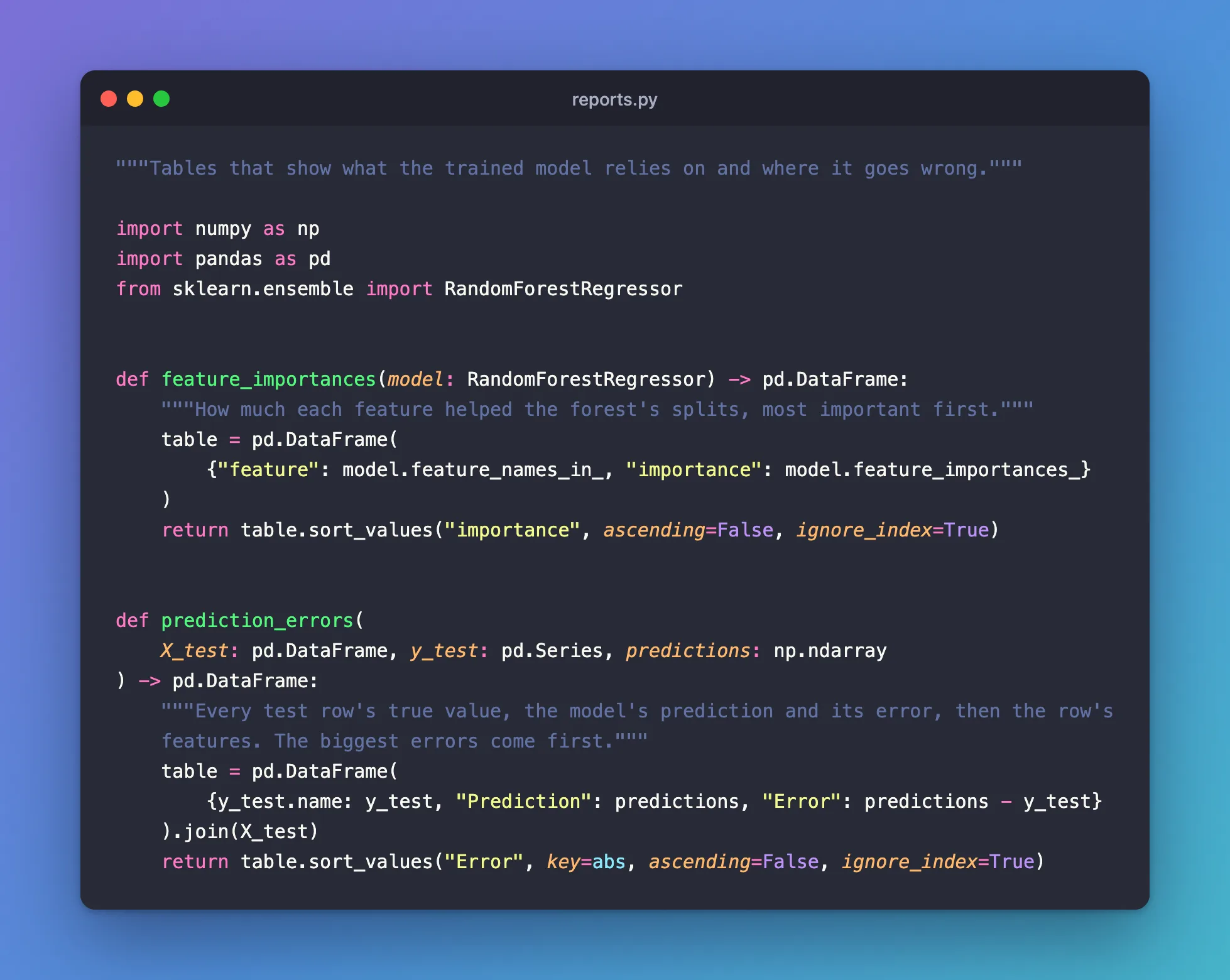
feature_importances reads two attributes of the trained forest: feature_names_in_, the column names, and feature_importances_, one share per feature that adds up to 1. How to Get Feature Importances from a Random Forest in scikit-learn explains what the shares mean. It pairs them in a table, built from a dictionary, and sorts it largest first, renumbering the rows.
prediction_errors builds one row per test district: the true value, the prediction and the error (prediction minus true value), followed by the district's features, so a spreadsheet shows the important columns first. key=abs sorts by the error's size whatever its sign, so the worst misses, too high or too low, come first.
The function is named prediction_errors, not test_predictions, for a practical reason: pytest collects any function whose name starts with test_ as a test once a test file imports it.
Step 6: Save the Table, the Settings and the CSV with the Run
Import the rest at the top of train.py:
import tempfile
from pathlib import Path

from house_price_prediction.reports import feature_importances, prediction_errors
Then, after Part 1's chart, save three files:
        mlflow.log_figure(figure, "plots/predicted_vs_actual.png")
        mlflow.log_table(feature_importances(model), "evaluation/feature_importances.json")
        mlflow.log_dict(model.get_params(), "model_params.json")
        with tempfile.TemporaryDirectory() as folder:
            csv_path = Path(folder) / "test_predictions.csv"
            errors = prediction_errors(data.X_test, data.y_test, predictions)
            errors.to_csv(csv_path, index=False)
            mlflow.log_artifact(csv_path, artifact_path="evaluation")
Each uses a different logging function, chosen for what happens to the file next:
| Line | What it saves | Why this function |
|---|---|---|
mlflow.log_table(...) | The importance table, as evaluation/feature_importances.json | MLflow marks it as a table: the UI shows it as rows and columns, compares it across runs, and mlflow.load_table() reads it back as a DataFrame |
mlflow.log_dict(model.get_params(), ...) | All 18 of the forest's settings, as model_params.json | Parameters hold the few settings you search by; this keeps every one, defaults included. How to See Every Setting of a scikit-learn Model with get_params |
The with block | The prediction errors, as evaluation/test_predictions.csv | log_artifact uploads a file that already exists, here a CSV anyone can open in a spreadsheet |
The CSV needs a file on disk first. tempfile.TemporaryDirectory() creates a fresh folder that Python deletes, file and all, when the block ends, so nothing is left in your project: How to Create a Temporary Folder in Python with tempfile. Path(folder) / "test_predictions.csv" builds the file's path, and to_csv(..., index=False) writes the table without its row numbers. artifact_path="evaluation" puts the file in the run's evaluation folder, next to the table.
The complete file:
"""Train a house price model and record the run in MLflow."""

import argparse
import logging
import tempfile
from collections.abc import Sequence
from pathlib import Path

import mlflow
from sklearn.ensemble import RandomForestRegressor
from sklearn.metrics import mean_absolute_error, r2_score, root_mean_squared_error

from house_price_prediction.config import get_settings
from house_price_prediction.data import load_housing_data, split_data
from house_price_prediction.datasets import split_datasets
from house_price_prediction.plots import predicted_vs_actual
from house_price_prediction.reports import feature_importances, prediction_errors

logger = logging.getLogger("house_price_prediction")


def parse_args(argv: Sequence[str] | None = None) -> argparse.Namespace:
    """Read the training options from the command line."""
    parser = argparse.ArgumentParser(
        prog="train",
        description="Train a model that predicts house prices, and track the run in MLflow.",
    )
    parser.add_argument(
        "--n-estimators", type=int, default=100, help="number of trees in the forest (default: 100)"
    )
    parser.add_argument(
        "--max-depth",
        type=int,
        default=None,
        help="how deep each tree may grow (default: no limit)",
    )
    parser.add_argument(
        "--trees-per-step",
        type=int,
        default=10,
        help="trees added between two validation scores (default: 10)",
    )
    parser.add_argument(
        "--test-size",
        type=float,
        default=0.2,
        help="share of the rows kept back for testing (default: 0.2)",
    )
    parser.add_argument(
        "--validation-size",
        type=float,
        default=0.2,
        help="share of the remaining rows used to score the model while it grows (default: 0.2)",
    )
    parser.add_argument(
        "--random-state",
        type=int,
        default=42,
        help="seed that makes the split and the model repeatable (default: 42)",
    )
    parser.add_argument(
        "--run-name", default=None, help="name shown in the MLflow UI (default: MLflow picks one)"
    )
    args = parser.parse_args(argv)
    if args.n_estimators < 1:
        parser.error("--n-estimators must be 1 or more")
    if args.max_depth is not None and args.max_depth < 1:
        parser.error("--max-depth must be 1 or more")
    if args.trees_per_step < 1:
        parser.error("--trees-per-step must be 1 or more")
    if not 0 < args.test_size < 1:
        parser.error("--test-size must be between 0 and 1")
    if not 0 < args.validation_size < 1:
        parser.error("--validation-size must be between 0 and 1")
    return args


def tree_counts(n_estimators: int, trees_per_step: int) -> list[int]:
    """The forest's size after each step: 10, 20, ... up to `n_estimators`."""
    counts = list(range(trees_per_step, n_estimators, trees_per_step))
    return [*counts, n_estimators]


def main(argv: Sequence[str] | None = None) -> int:
    """Grow the forest step by step, score each step on the validation rows, then measure the
    finished model on the test rows. Everything goes into one MLflow run."""
    logging.basicConfig(
        level=logging.INFO,
        format="%(asctime)s %(levelname)s %(name)s: %(message)s",
        datefmt="%Y/%m/%d %H:%M:%S",
    )
    args = parse_args(argv)
    settings = get_settings()

    mlflow.set_tracking_uri(settings.mlflow_tracking_uri)
    mlflow.set_experiment(settings.mlflow_experiment_name)
    mlflow.set_system_metrics_sampling_interval(settings.system_metrics_interval)

    logger.info("Loading the California Housing data")
    data = split_data(load_housing_data(), args.test_size, args.validation_size, args.random_state)

    with mlflow.start_run(
        run_name=args.run_name, log_system_metrics=settings.log_system_metrics
    ) as run:
        mlflow.log_params(
            {
                "n_estimators": args.n_estimators,
                "max_depth": args.max_depth,
                "trees_per_step": args.trees_per_step,
                "test_size": args.test_size,
                "validation_size": args.validation_size,
                "random_state": args.random_state,
            }
        )
        mlflow.set_tags({"model_type": "random_forest", "dataset": "california_housing"})
        for context, dataset in split_datasets(data).items():
            mlflow.log_input(dataset, context=context)

        model = RandomForestRegressor(
            max_depth=args.max_depth,
            random_state=args.random_state,
            n_jobs=-1,
            warm_start=True,
        )
        logger.info(
            "Training on %d rows, scoring on %d validation rows", len(data.X_train), len(data.X_val)
        )
        for n_trees in tree_counts(args.n_estimators, args.trees_per_step):
            model.set_params(n_estimators=n_trees)
            model.fit(data.X_train, data.y_train)
            val_predictions = model.predict(data.X_val)
            val_metrics = {
                "val_mae": mean_absolute_error(data.y_val, val_predictions),
                "val_rmse": root_mean_squared_error(data.y_val, val_predictions),
                "val_r2": r2_score(data.y_val, val_predictions),
            }
            mlflow.log_metrics(val_metrics, step=n_trees)
            logger.info("%4d trees: validation RMSE %.4f", n_trees, val_metrics["val_rmse"])

        predictions = model.predict(data.X_test)
        metrics = {
            "mae": mean_absolute_error(data.y_test, predictions),
            "rmse": root_mean_squared_error(data.y_test, predictions),
            "r2": r2_score(data.y_test, predictions),
        }
        mlflow.log_metrics(metrics)
        figure = predicted_vs_actual(data.y_test.to_numpy(), predictions)
        mlflow.log_figure(figure, "plots/predicted_vs_actual.png")
        mlflow.log_table(feature_importances(model), "evaluation/feature_importances.json")
        mlflow.log_dict(model.get_params(), "model_params.json")
        with tempfile.TemporaryDirectory() as folder:
            csv_path = Path(folder) / "test_predictions.csv"
            errors = prediction_errors(data.X_test, data.y_test, predictions)
            errors.to_csv(csv_path, index=False)
            mlflow.log_artifact(csv_path, artifact_path="evaluation")

        logger.info(
            "Run %s: MAE %.3f, RMSE %.3f, R2 %.3f",
            run.info.run_name,
            metrics["mae"],
            metrics["rmse"],
            metrics["r2"],
        )
    return 0
Step 7: Train Three Forests
Three runs make the comparisons in the next steps meaningful: Part 2's default forest, a shallower one trained on the same data, and the default forest trained on a different split, from another --random-state:
uv run train --run-name seed-42-100-trees
2026/11/19 16:10:14 INFO house_price_prediction: Loading the California Housing data
2026/11/19 16:10:14 INFO mlflow.system_metrics.system_metrics_monitor: Skip logging GPU metrics. Set logger level to DEBUG for more details.
2026/11/19 16:10:14 INFO mlflow.system_metrics.system_metrics_monitor: Started monitoring system metrics.
2026/11/19 16:10:14 INFO house_price_prediction: Training on 13209 rows, scoring on 3303 validation rows
2026/11/19 16:10:14 INFO house_price_prediction:   10 trees: validation RMSE 0.5490
2026/11/19 16:10:14 INFO house_price_prediction:   20 trees: validation RMSE 0.5417
2026/11/19 16:10:14 INFO house_price_prediction:   30 trees: validation RMSE 0.5363
2026/11/19 16:10:14 INFO house_price_prediction:   40 trees: validation RMSE 0.5320
2026/11/19 16:10:15 INFO house_price_prediction:   50 trees: validation RMSE 0.5308
2026/11/19 16:10:15 INFO house_price_prediction:   60 trees: validation RMSE 0.5300
2026/11/19 16:10:15 INFO house_price_prediction:   70 trees: validation RMSE 0.5301
2026/11/19 16:10:15 INFO house_price_prediction:   80 trees: validation RMSE 0.5287
2026/11/19 16:10:15 INFO house_price_prediction:   90 trees: validation RMSE 0.5283
2026/11/19 16:10:15 INFO house_price_prediction:  100 trees: validation RMSE 0.5276
2026/11/19 16:10:15 INFO house_price_prediction: Run seed-42-100-trees: MAE 0.337, RMSE 0.516, R2 0.797
🏃 View run seed-42-100-trees at: http://127.0.0.1:8080/#/experiments/1/runs/175b697b4d2c4370b6d9f210d64e20be
🧪 View experiment at: http://127.0.0.1:8080/#/experiments/1
2026/11/19 16:10:15 INFO mlflow.system_metrics.system_metrics_monitor: Stopping system metrics monitoring...
2026/11/19 16:10:15 INFO mlflow.system_metrics.system_metrics_monitor: Successfully terminated system metrics monitoring!
The same scores as Part 2's curve-100-trees, MAE 0.337, RMSE 0.516 and R² 0.797: same data, same seed, same forest. The new logging adds no lines to the output. Now the other two:
uv run train --run-name seed-42-depth-8 --max-depth 8
uv run train --run-name seed-7-100-trees --random-state 7
2026/11/19 16:10:18 INFO house_price_prediction: Loading the California Housing data
2026/11/19 16:10:18 INFO mlflow.system_metrics.system_metrics_monitor: Skip logging GPU metrics. Set logger level to DEBUG for more details.
2026/11/19 16:10:18 INFO mlflow.system_metrics.system_metrics_monitor: Started monitoring system metrics.
2026/11/19 16:10:18 INFO house_price_prediction: Training on 13209 rows, scoring on 3303 validation rows
2026/11/19 16:10:18 INFO house_price_prediction:   10 trees: validation RMSE 0.5939
2026/11/19 16:10:18 INFO house_price_prediction:   20 trees: validation RMSE 0.5922
2026/11/19 16:10:19 INFO house_price_prediction:   30 trees: validation RMSE 0.5888
2026/11/19 16:10:19 INFO house_price_prediction:   40 trees: validation RMSE 0.5875
2026/11/19 16:10:19 INFO house_price_prediction:   50 trees: validation RMSE 0.5875
2026/11/19 16:10:19 INFO house_price_prediction:   60 trees: validation RMSE 0.5867
2026/11/19 16:10:19 INFO house_price_prediction:   70 trees: validation RMSE 0.5872
2026/11/19 16:10:19 INFO house_price_prediction:   80 trees: validation RMSE 0.5862
2026/11/19 16:10:19 INFO house_price_prediction:   90 trees: validation RMSE 0.5861
2026/11/19 16:10:19 INFO house_price_prediction:  100 trees: validation RMSE 0.5857
2026/11/19 16:10:19 INFO house_price_prediction: Run seed-42-depth-8: MAE 0.403, RMSE 0.586, R2 0.738
🏃 View run seed-42-depth-8 at: http://127.0.0.1:8080/#/experiments/1/runs/1bc28a52be544b08a01bd133014a36cb
🧪 View experiment at: http://127.0.0.1:8080/#/experiments/1
2026/11/19 16:10:19 INFO mlflow.system_metrics.system_metrics_monitor: Stopping system metrics monitoring...
2026/11/19 16:10:19 INFO mlflow.system_metrics.system_metrics_monitor: Successfully terminated system metrics monitoring!
2026/11/19 16:10:22 INFO house_price_prediction: Loading the California Housing data
2026/11/19 16:10:22 INFO mlflow.system_metrics.system_metrics_monitor: Skip logging GPU metrics. Set logger level to DEBUG for more details.
2026/11/19 16:10:22 INFO mlflow.system_metrics.system_metrics_monitor: Started monitoring system metrics.
2026/11/19 16:10:22 INFO house_price_prediction: Training on 13209 rows, scoring on 3303 validation rows
2026/11/19 16:10:22 INFO house_price_prediction:   10 trees: validation RMSE 0.5359
2026/11/19 16:10:22 INFO house_price_prediction:   20 trees: validation RMSE 0.5206
2026/11/19 16:10:23 INFO house_price_prediction:   30 trees: validation RMSE 0.5182
2026/11/19 16:10:23 INFO house_price_prediction:   40 trees: validation RMSE 0.5151
2026/11/19 16:10:23 INFO house_price_prediction:   50 trees: validation RMSE 0.5157
2026/11/19 16:10:23 INFO house_price_prediction:   60 trees: validation RMSE 0.5153
2026/11/19 16:10:23 INFO house_price_prediction:   70 trees: validation RMSE 0.5148
2026/11/19 16:10:23 INFO house_price_prediction:   80 trees: validation RMSE 0.5144
2026/11/19 16:10:23 INFO house_price_prediction:   90 trees: validation RMSE 0.5142
2026/11/19 16:10:23 INFO house_price_prediction:  100 trees: validation RMSE 0.5132
2026/11/19 16:10:23 INFO house_price_prediction: Run seed-7-100-trees: MAE 0.344, RMSE 0.526, R2 0.794
🏃 View run seed-7-100-trees at: http://127.0.0.1:8080/#/experiments/1/runs/71fd7f2ea29145f6adf4d43e99c46a9d
🧪 View experiment at: http://127.0.0.1:8080/#/experiments/1
2026/11/19 16:10:23 INFO mlflow.system_metrics.system_metrics_monitor: Stopping system metrics monitoring...
2026/11/19 16:10:23 INFO mlflow.system_metrics.system_metrics_monitor: Successfully terminated system metrics monitoring!
- The depth-8 forest scores worse, as in Part 2: test RMSE 0.586.
- The seed-7 forest has a better validation score than the seed-42 one, 0.5132 against 0.5276, but a worse test score, 0.526 against 0.516. It wasn't scored on the same rows:
--random-state 7split the data differently. The datasets will show it.
Your times and run IDs will differ.
Step 8: See Which Data Each Run Used
Open the house-price-prediction experiment in the MLflow UI at http://127.0.0.1:8080. The runs table has a Dataset column; with three datasets per run it's cut short, so turn on Expand rows above the table. Widen the column by dragging its right edge if the labels are cut off:
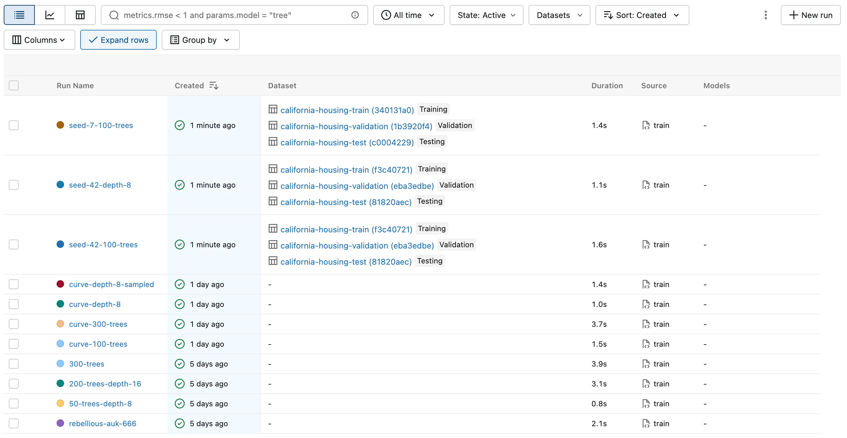
- The two seed-42 runs show the same three digests,
f3c40721,eba3edbeand81820aec: they learned from, were checked against and were tested on identical data. Their scores can be compared fairly, and the depth limit is the only difference. - The seed-7 run shows three different digests. Its better validation score came from different validation rows, so it says nothing about which forest is better.
- Parts 1 and 2's runs show
-: they logged no datasets.
The Datasets button in the toolbar lists every dataset by name and digest; tick one to show only the runs that used it. How to Check Whether Two MLflow Runs Used the Same Data does the same check in Python.
Click a dataset's name, such as california-housing-train (f3c40721) in the seed-42-100-trees row:
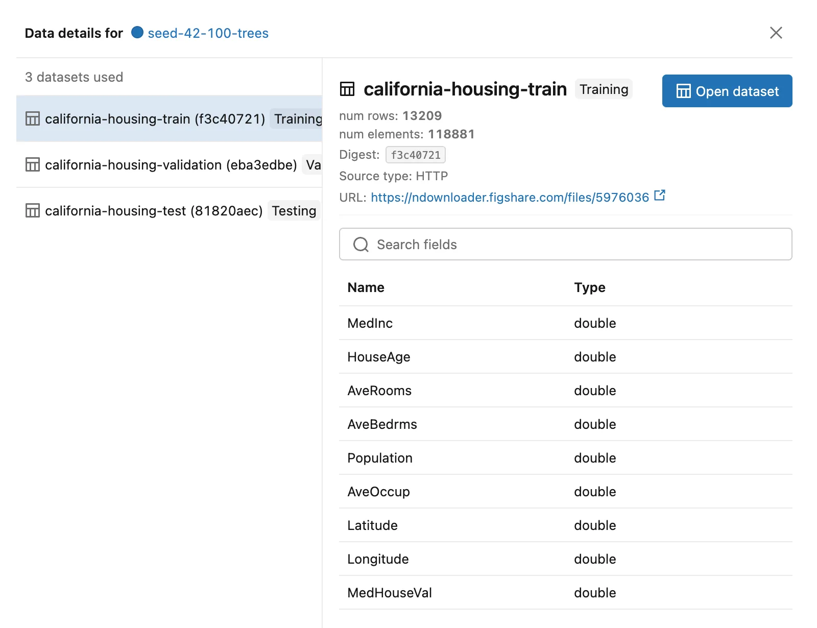
The panel shows what the run recorded about its training data: 13,209 rows, 118,881 values (13,209 rows of 9 columns), the digest, the source with a link to it, and all nine columns with their type, double. Open dataset opens the source address in a new tab, which downloads the original archive. The run's own page lists the same datasets under About this run:
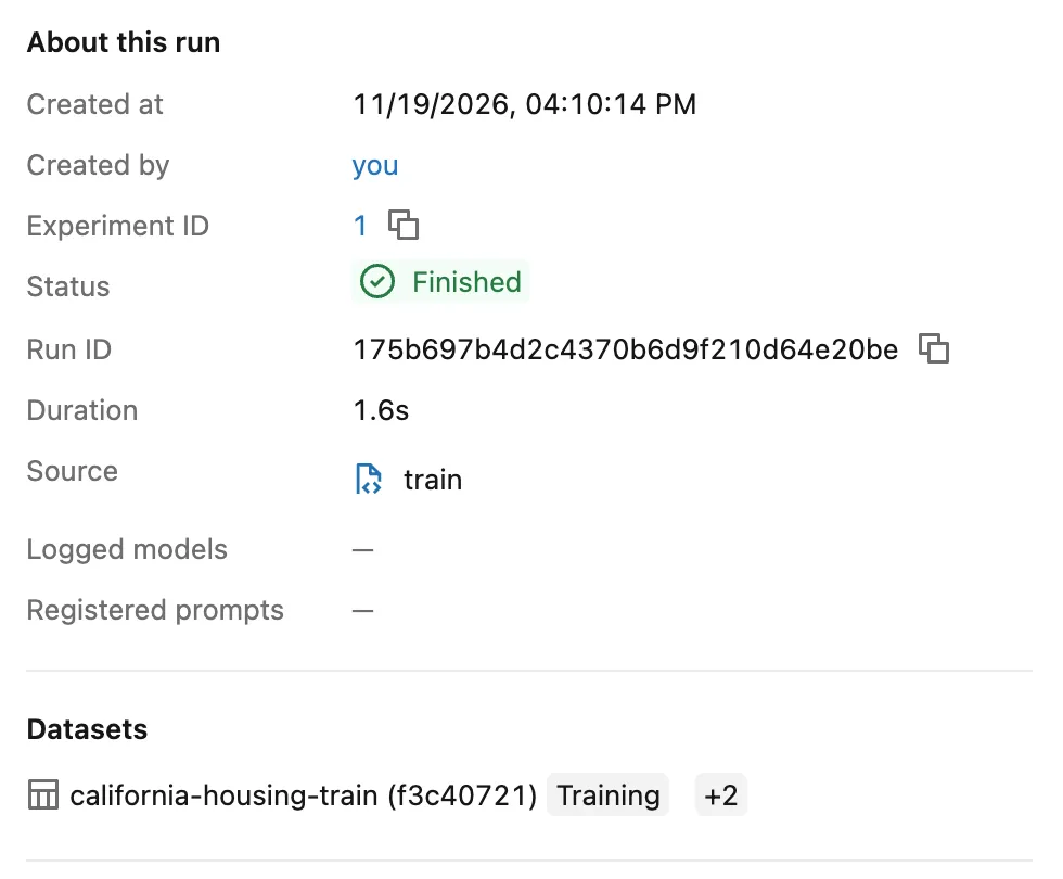
Click +2 for the validation and test sets.
Step 9: Open the Run's Files
On the seed-42-100-trees run page, click Artifacts. Next to Part 1's plots folder are the new files: evaluation with the table and the CSV, and model_params.json. Expand evaluation and click feature_importances.json:
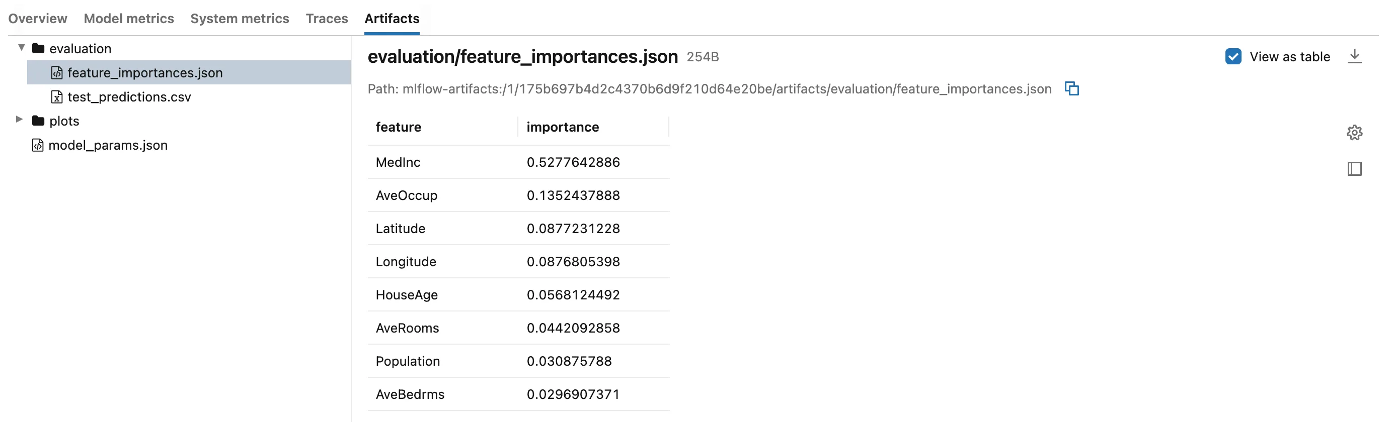
Because log_table saved it, the preview has View as table. The median income (MedInc) accounts for 53% of the forest's error reduction, household size (AveOccup) for 14%, and the location for about 9% per coordinate.
Click model_params.json:
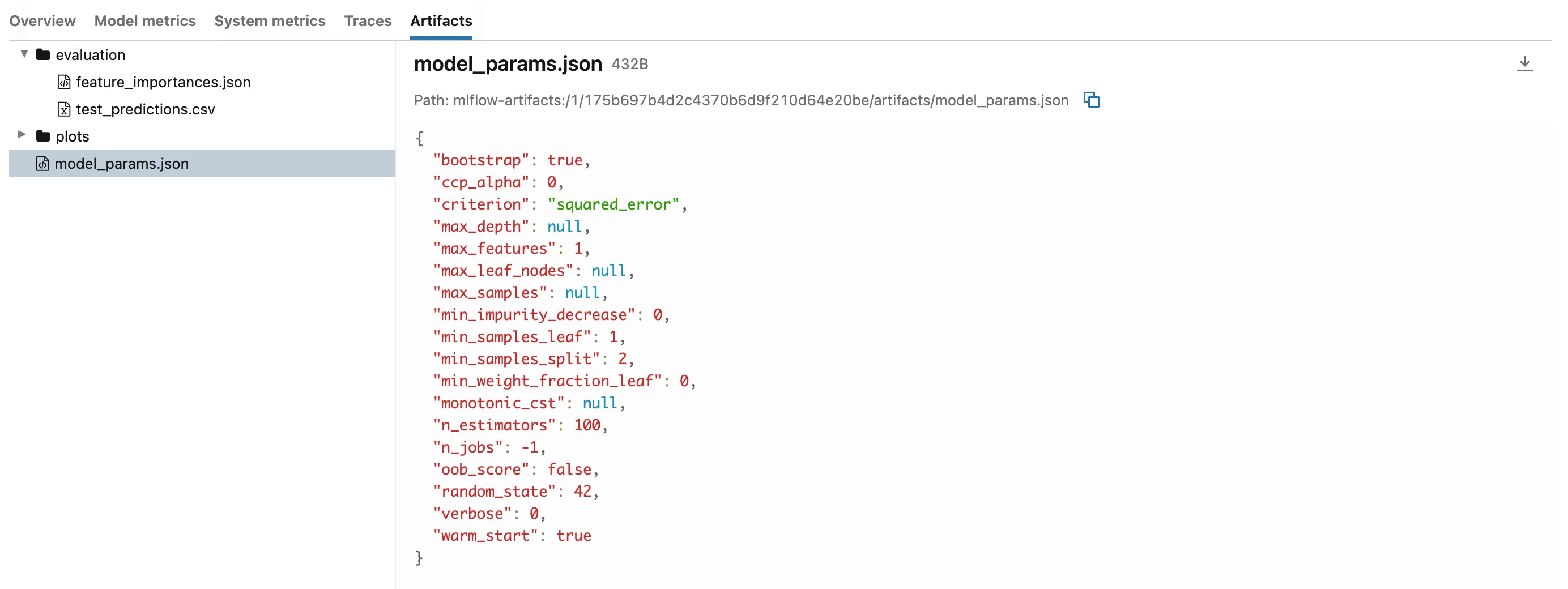
All 18 settings, including the 13 the code never sets, such as max_features and min_samples_leaf. The run's parameters still hold the six chosen on the command line. The file also shows warm_start: true and n_jobs: -1 from the code, and n_estimators: 100, the forest's final size after the last stage.
Click test_predictions.csv:
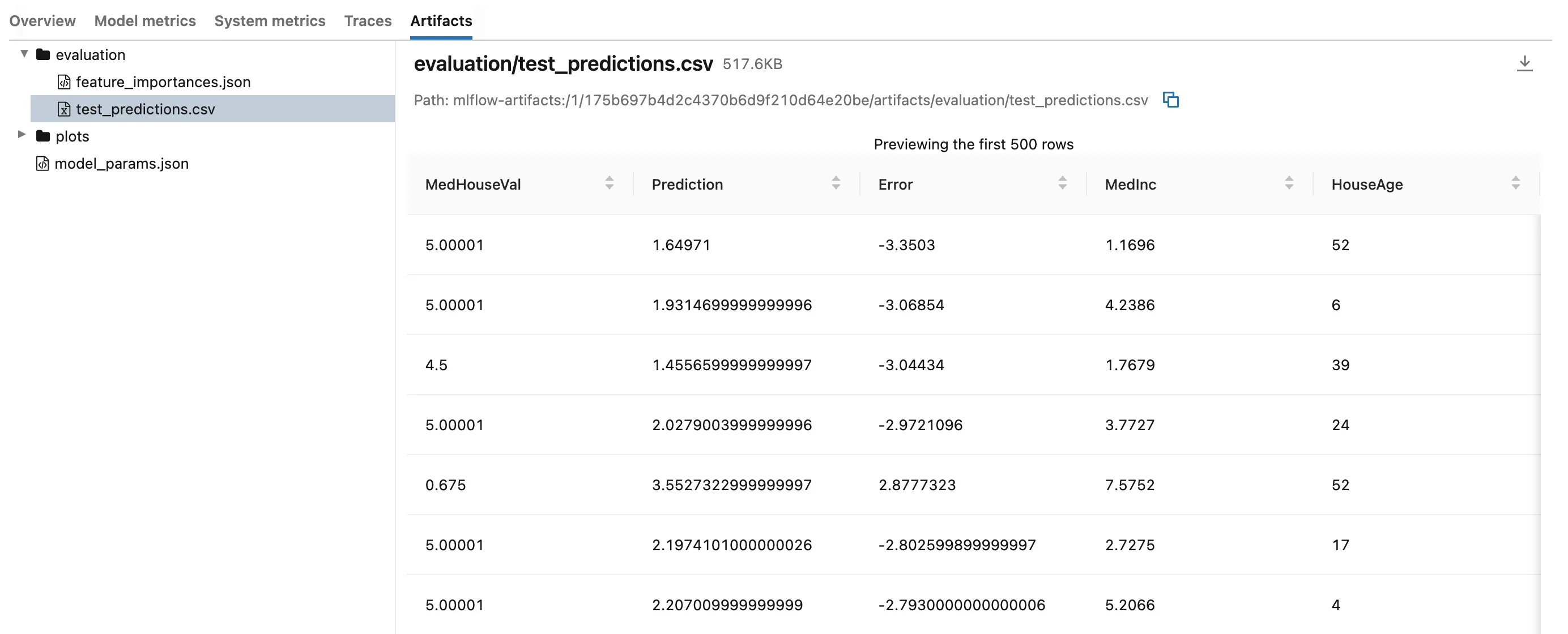
The CSV has all 4,128 test districts, and the preview shows the first 500, biggest misses first. Six of the ten biggest misses are districts whose true value is 5.00001, the highest value in the test rows, which the forest predicts far lower. That's the kind of pattern this file is for: open it in a spreadsheet, or with pandas, to see where the model fails.
Step 10: Compare the Files Across Runs
Two places compare files between runs. For tables logged with log_table, the experiment's runs page has a third view: click the Artifact evaluation button next to the table and chart buttons. Table picks evaluation/feature_importances.json, Group by feature and Compare importance:
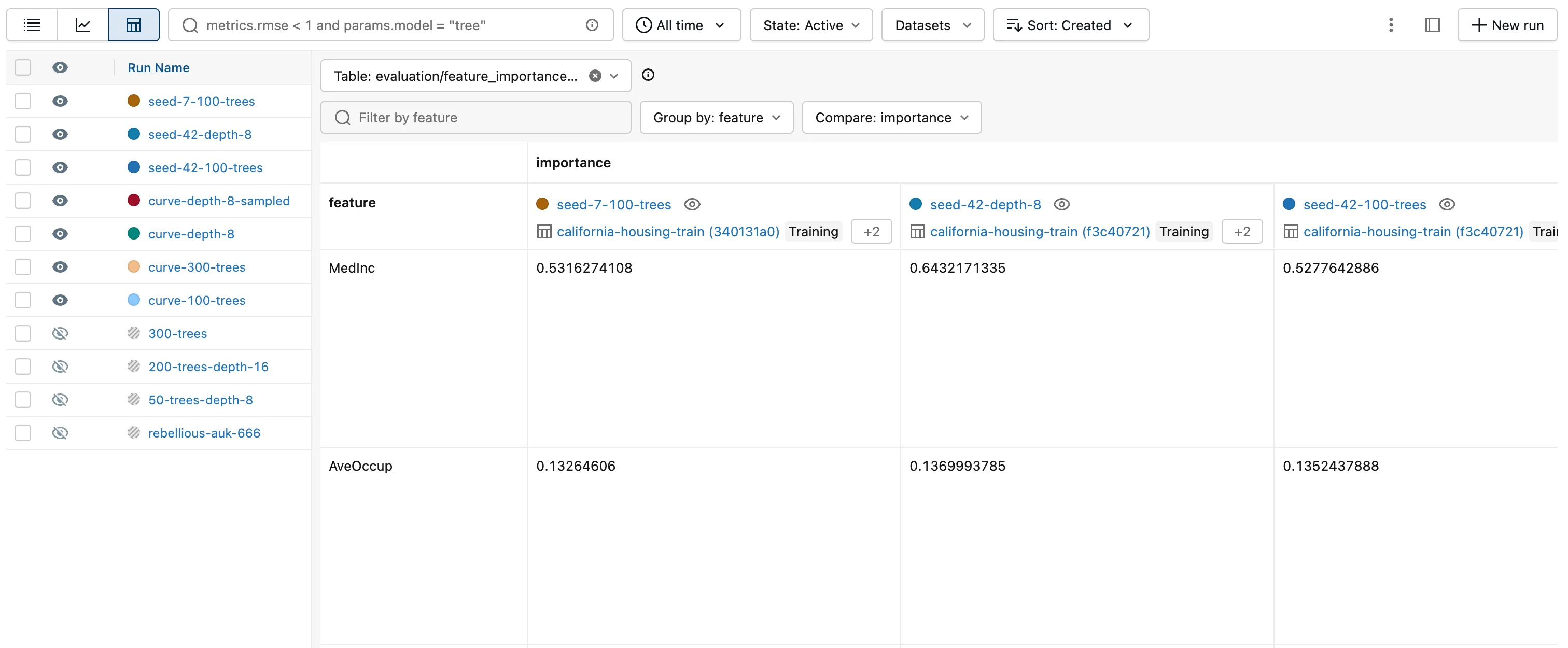
The shallow forest leans even harder on income, 64% against 53%, and less on the location. Only runs that logged the table get a column. How to Compare a Logged Table Across Runs in the MLflow UI covers the view's other controls.
For any other file, select runs in the runs table and click Compare. Near the bottom, the Artifacts section lists the files at the top level of the runs, model_params.json here; click it:
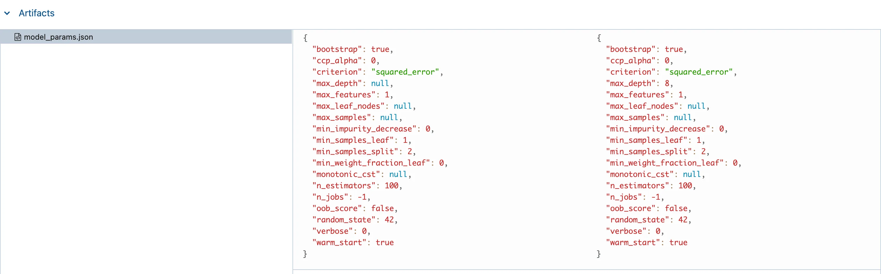
The two seed-42 forests differ in exactly one setting, max_depth. The section lists only top-level files, which is one reason model_params.json sits outside the evaluation folder.
Step 11: Save Your Work with Git
git status --short --untracked-files=all
 M src/house_price_prediction/data.py
 M src/house_price_prediction/train.py
?? src/house_price_prediction/datasets.py
?? src/house_price_prediction/reports.py
Two changed files and two new ones. The CSV was written to a temporary folder, so nothing else appears. Commit them:
git add .
git commit -m "Record each run's datasets and evaluation files"
[master c4224c2] Record each run's datasets and evaluation files
 4 files changed, 62 insertions(+)
 create mode 100644 src/house_price_prediction/datasets.py
 create mode 100644 src/house_price_prediction/reports.py
Your commit ID will differ.
Your Folders Now Look Like This
source/
├── mlflow-server/
│   ├── .venv/
│   ├── mlartifacts/
│   ├── mlflow.db
│   ├── pyproject.toml
│   └── uv.lock
└── dewiride-house-price-prediction/
    ├── .venv/
    ├── src/
    │   └── house_price_prediction/
    │       ├── __init__.py
    │       ├── config.py
    │       ├── curve.py
    │       ├── data.py
    │       ├── datasets.py
    │       ├── plots.py
    │       ├── reports.py
    │       └── train.py
    ├── .env
    ├── .env.example
    ├── .gitignore
    ├── .python-version
    ├── README.md
    ├── pyproject.toml
    └── uv.lock
The files went to mlflow-server/mlartifacts/1/<run ID>/artifacts/, next to Part 1's chart. The dataset records went into mlflow.db, with no copy of the data.
Do It with the CLI
The same files are a command away. The mlflow command reads the server's address from MLFLOW_TRACKING_URI, which your project's .env file already holds; --env-file .env loads it, the same way in every shell. List a run's files, using your own run ID:
uv run mlflow --env-file .env artifacts list --run-id 175b697b4d2c4370b6d9f210d64e20be
Loaded environment variables from: .env
[{
  "path": "evaluation",
  "is_dir": true
}, {
  "path": "model_params.json",
  "is_dir": false,
  "file_size": 432
}, {
  "path": "plots",
  "is_dir": true
}]
One level at a time. Look inside evaluation:
uv run mlflow --env-file .env artifacts list --run-id 175b697b4d2c4370b6d9f210d64e20be --artifact-path evaluation
Loaded environment variables from: .env
[{
  "path": "evaluation/feature_importances.json",
  "is_dir": false,
  "file_size": 254
}, {
  "path": "evaluation/test_predictions.csv",
  "is_dir": false,
  "file_size": 530018
}]
And download the folder next to your project, so the files stay out of Git:
uv run mlflow --env-file .env artifacts download --run-id 175b697b4d2c4370b6d9f210d64e20be --artifact-path evaluation --dst-path ../downloads
Loaded environment variables from: .env

/Users/you/source/downloads/evaluation
The command prints where it put the folder. How to Download Artifacts from an MLflow Run shows the same from Python. Delete the downloads folder when you no longer need it.
Stop the Server When You're Done
Go to the first terminal and press Ctrl+C. Your runs, datasets and files stay in mlflow.db and mlartifacts/, and uv run mlflow server --port 8080 in the mlflow-server folder brings them back.
Keep both folders for Part 4. If you ever want to remove everything the series created, stop the server first, then delete the mlflow-server and dewiride-house-price-prediction folders, and the scikit_learn_data folder in your home folder.
Common Mistakes
| Mistake | What happens | Do this instead |
|---|---|---|
| Comparing runs' scores without checking their datasets | Runs tested on different rows look better or worse for the wrong reason, like seed-7-100-trees here | Check that the digests match first |
| Expecting the dataset record to contain the data | The run holds a description: digest, schema, row count and source | Keep the data where source points, or log the file itself as an artifact |
Logging the importance table with log_artifact | The UI shows plain JSON, and the table can't be compared across runs | Use log_table for tables |
| Writing the CSV into the project folder | It shows up in git status and gets committed by accident | Write it into a temporary folder, as in Step 6 |
| Putting a file you want to compare inside a folder | The compare page lists only top-level files | Log it at the top level, as model_params.json is |
Troubleshooting
| Symptom | Likely cause | Fix |
|---|---|---|
The Dataset column shows - for new runs | log_input wasn't reached, or runs were trained with the old code | Check Step 4's lines and train again |
MlflowException: The specified pandas DataFrame does not contain the specified targets column 'MedHouseVal'. | The target wasn't joined to the features | Pass features.join(target) to from_pandas, as in Step 3 |
ValueError: Invalid artifact file path ... '.json' or '.parquet' extension | log_table was given another extension | Name the table .json |
pytest prints Pandas4Warning: For backward compatibility, 'str' dtypes are included by select_dtypes | MLflow's log_table with pandas 3, in tests | Fixed: Pandas4Warning in MLflow log_table |
pytest reports ERROR for a function called test_predictions | A function whose name starts with test_ was imported into a test file, so pytest collected it as a test | Name it something else, such as prediction_errors |
FAQ
Why not store the data itself with every run?
The training set is 13,209 rows, and real projects have far bigger ones; copying it into every run would fill the artifact store. The digest is enough to tell whether two runs used the same data, and the source says where to get it. When a dataset can't be fetched again, log the file as an artifact as well.
Does the digest catch every change to the data?
For a pandas table, MLflow fingerprints the text and number columns of the first 10,000 rows, plus the row count and the column names. The training set has 13,209 rows, so a change in its last 3,209 rows that keeps the row count wouldn't change it. How to Make an MLflow Dataset Digest Cover Every Row shows how to fingerprint every row.
Can I read the feature importances of several runs in Python?
Yes: mlflow.load_table("evaluation/feature_importances.json", extra_columns=["tags.mlflow.runName"]) stacks them from every run of the experiment, labelled by run name: How to Load a Logged Table from MLflow with load_table.
Why do the CSV's predictions have so many decimals?
Each prediction is the average of 100 trees, written with every digit Python keeps. The values are exact; round them in your spreadsheet if you prefer.
Conclusion
Every run now records its data and keeps its files. mlflow.data.from_pandas() and mlflow.log_input() attach the training, validation and test sets with their digests, so the UI shows at a glance that the two seed-42 runs used identical data and the seed-7 run didn't. log_table saved the feature importances as a table the UI compares across runs, log_dict kept all 18 of the forest's settings, and log_artifact uploaded a CSV of every test prediction, which showed that the forest misses most on the highest-valued districts.
In Part 4 you'll search runs by their parameters, metrics, tags and datasets, in the UI and from Python.
Additional Resources
- MLflow Dataset Tracking — MLflow's guide to
mlflow.dataandlog_input. - mlflow.log_table, mlflow.log_dict and mlflow.log_artifact — the three logging functions.
- mlflow artifacts — the command-line reference, including
listanddownload.
← Previous: Part 2: Log Metrics Over Time and System Metrics
Next → Part 4: Search and Filter Runs (coming soon)
