MLflow Tutorial for Machine Learning in Python — Part 2: Log Metrics Over Time and System Metrics

Part 1 logged each score once, after training was over. That hides the question every model raises: was more training still helping? In this part the forest grows in stages, MLflow records its score after every stage, and the curves show where extra trees stop paying off. MLflow also records how hard the computer worked while it trained.
This is Part 2 of a 9-part series.
- Part 1: Install MLflow and Track Your First Experiment
- Part 2: Log Metrics Over Time and System Metrics (you are here)
- Part 3: Log Artifacts and Datasets (coming soon)
- Part 4: Autologging and Hyperparameter Tuning with Nested Runs (coming soon)
- Part 5: Log, Load and Validate Models (coming soon)
- Part 6: Evaluate Models and Set Quality Gates (coming soon)
- Part 7: Register, Version and Promote Models with the Model Registry (coming soon)
- Part 8: Serve a Model as a REST API and in Docker (coming soon)
- Part 9: Production Checklist and Recap (coming soon)
Every command and output on this page is real, captured while building the project.
What You'll Build in This Part
You'll keep working on Part 1's house price project and add:
- a validation set, a third slice of the data, to score the model while it trains without touching the test rows;
- a forest that grows in stages, 10 trees at a time, with three validation scores logged after each stage at a step equal to the number of trees so far;
- learning curves in the MLflow UI, for one run and for three runs side by side;
- a
curvecommand that reads a run's curve back from MLflow and names its best step; - system metrics: the computer's CPU, memory, disk and network use, sampled every second during each run.
What This Part Costs
Nothing. Everything still runs on your own computer, and the one new package, psutil, is free and open source.
Prerequisites
- Part 1 finished: the
mlflow-serverfolder with its runs, and thedewiride-house-price-predictionproject, committed to Git. Part 1 builds both. - The same tools as Part 1: Python 3.15 and uv 0.13.9 or newer.
Each technique this part uses also has a short guide of its own, linked where it comes up.
Step 1: Start the Tracking Server
Open a terminal in the mlflow-server folder and start the server, as in Part 1:
uv run mlflow server --port 8080
Wait until it prints Application startup complete, and leave it running. Open a second terminal in the dewiride-house-price-prediction folder for everything else.
Step 2: Split Off a Validation Set
Part 1 split the rows in two: 80% to train on and 20% to test. To watch the score while the forest grows, you need rows the model doesn't learn from, and the test rows can't do that job: once you choose the number of trees by looking at the test score, that score is no longer a fair check on data the model has never seen. So this part takes a third slice out of the training rows, the validation set, and keeps the test rows for one final score at the end. How to Split Data into Training, Validation and Test Sets with scikit-learn explains the idea on its own.
Open src/house_price_prediction/data.py. Give DataSplit two more fields, for the validation rows and their prices:
@dataclass(frozen=True)
class DataSplit:
    """The features and target values for training, validation and testing."""

    X_train: pd.DataFrame
    X_val: pd.DataFrame
    X_test: pd.DataFrame
    y_train: pd.Series
    y_val: pd.Series
    y_test: pd.Series
Split twice. Replace split_data with:
def split_data(
    frame: pd.DataFrame, test_size: float, validation_size: float, random_state: int
) -> DataSplit:
    """Hold back `test_size` of the rows for the final test, then `validation_size` of the rest
    to watch the model while it trains. The model learns from what is left."""
    features = frame.drop(columns=TARGET)
    target = frame[TARGET]
    X_rest, X_test, y_rest, y_test = train_test_split(
        features, target, test_size=test_size, random_state=random_state
    )
    X_train, X_val, y_train, y_val = train_test_split(
        X_rest, y_rest, test_size=validation_size, random_state=random_state
    )
    return DataSplit(X_train, X_val, X_test, y_train, y_val, y_test)
- The first split is Part 1's, with the same
test_sizeandrandom_state, so the test set is the same 4,128 rows as before. - The second split takes
validation_sizeof the remaining 16,512 rows for validation: with 0.2, that's 3,303 rows, which leaves 13,209 to train on.
The complete file, with its first line updated too:
"""Load the California Housing data and split it for training, validation and testing."""

from dataclasses import dataclass

import pandas as pd
from sklearn.datasets import fetch_california_housing
from sklearn.model_selection import train_test_split

TARGET = "MedHouseVal"


@dataclass(frozen=True)
class DataSplit:
    """The features and target values for training, validation and testing."""

    X_train: pd.DataFrame
    X_val: pd.DataFrame
    X_test: pd.DataFrame
    y_train: pd.Series
    y_val: pd.Series
    y_test: pd.Series


def load_housing_data() -> pd.DataFrame:
    """Return the dataset as one table. The first call downloads it; later calls read a cache."""
    return fetch_california_housing(as_frame=True).frame


def split_data(
    frame: pd.DataFrame, test_size: float, validation_size: float, random_state: int
) -> DataSplit:
    """Hold back `test_size` of the rows for the final test, then `validation_size` of the rest
    to watch the model while it trains. The model learns from what is left."""
    features = frame.drop(columns=TARGET)
    target = frame[TARGET]
    X_rest, X_test, y_rest, y_test = train_test_split(
        features, target, test_size=test_size, random_state=random_state
    )
    X_train, X_val, y_train, y_val = train_test_split(
        X_rest, y_rest, test_size=validation_size, random_state=random_state
    )
    return DataSplit(X_train, X_val, X_test, y_train, y_val, y_test)
Step 3: Add the System Metrics Settings
System metrics are MLflow's record of the computer itself while a run works: how busy the processor is, how much memory is in use, and how much the disk and network move. They show whether training is starved for memory or using every core. MLflow samples them every 10 seconds by default, but each training run here takes a few seconds, and a run that ends before its first sample is logged records nothing. So the project samples every second, and both choices become settings you can change without touching the code. How to Turn On System Metrics Logging in MLflow and How to Change the System Metrics Sampling Interval in MLflow cover both settings on their own.
Open src/house_price_prediction/config.py and add two settings at the end of the Settings class:
    log_system_metrics: bool = Field(
        default=True,
        description="Record the computer's CPU, memory, disk and network use during each run.",
    )
    system_metrics_interval: float = Field(
        default=1.0,
        ge=0.1,
        description="Seconds between two system metrics samples. A run records nothing unless it "
        "lasts longer than one interval, so keep this below your shortest run.",
    )
- pydantic-settings reads them from the environment variables
HOUSE_PRICES_LOG_SYSTEM_METRICSandHOUSE_PRICES_SYSTEM_METRICS_INTERVAL: the class'senv_prefix,HOUSE_PRICES_, plus the field's name. How to Load Settings from Environment Variables and a .env File with pydantic-settings explains the prefix. ge=0.1refuses an interval shorter than 0.1 seconds. psutil, the package MLflow reads CPU use with, recommends at least that much time between two readings for accuracy.
The complete file:
"""Settings, read from environment variables and the .env file."""

from functools import lru_cache

from pydantic import Field
from pydantic_settings import BaseSettings, SettingsConfigDict


class Settings(BaseSettings):
    """Where the project sends its MLflow runs, and what each run records about the computer."""

    model_config = SettingsConfigDict(
        env_prefix="HOUSE_PRICES_",
        env_file=".env",
        env_file_encoding="utf-8",
        extra="ignore",
    )

    mlflow_tracking_uri: str = Field(
        default="http://127.0.0.1:8080",
        validation_alias="MLFLOW_TRACKING_URI",
        description="The address of the MLflow tracking server.",
    )
    mlflow_experiment_name: str = Field(
        default="house-price-prediction",
        min_length=1,
        validation_alias="MLFLOW_EXPERIMENT_NAME",
        description="The MLflow experiment that groups this project's runs.",
    )
    log_system_metrics: bool = Field(
        default=True,
        description="Record the computer's CPU, memory, disk and network use during each run.",
    )
    system_metrics_interval: float = Field(
        default=1.0,
        ge=0.1,
        description="Seconds between two system metrics samples. A run records nothing unless it "
        "lasts longer than one interval, so keep this below your shortest run.",
    )


@lru_cache
def get_settings() -> Settings:
    """Read the settings once, then reuse the same object everywhere."""
    return Settings()
Then document the new settings for whoever uses the project next. Add these lines at the end of .env.example:
# Record the computer's CPU, memory, disk and network use during each run (true or false).
HOUSE_PRICES_LOG_SYSTEM_METRICS=true
# Seconds between two system metrics samples (0.1 or more). A run records none unless it lasts
# longer than one interval, so keep this below your shortest training run.
HOUSE_PRICES_SYSTEM_METRICS_INTERVAL=1
Your own .env needs no change: a setting that's missing there takes its default from config.py, and the defaults are the same values.
Step 4: Grow the Forest in Stages and Log a Score at Every Step
This is the heart of the part. A random forest averages the answers of many decision trees. Part 1 grew all its trees in one go and scored the finished forest once. Now the forest grows 10 trees, gets scored on the validation rows, grows 10 more, gets scored again, and so on. Two settings make that work:
warm_start=Truetells scikit-learn to keep the trees it already has when you raisen_estimatorsand callfitagain, so each stage adds trees instead of starting over: How to Use warm_start to Add Trees to a Random Forest in scikit-learn.step=inmlflow.log_metrics()records each score together with a whole number you choose. A metric logged at several steps becomes a curve: MLflow keeps every value with its step, and the UI draws them as a line. Here the step is the number of trees, so the curve reads in trees. How to Log Metrics in MLflow introducedstep.
Open src/house_price_prediction/train.py and change it piece by piece.
Two new options. In parse_args, add --trees-per-step below --max-depth, and --validation-size below --test-size:
    parser.add_argument(
        "--trees-per-step",
        type=int,
        default=10,
        help="trees added between two validation scores (default: 10)",
    )
    parser.add_argument(
        "--validation-size",
        type=float,
        default=0.2,
        help="share of the remaining rows used to score the model while it grows (default: 0.2)",
    )
Check both. The checks at the end of parse_args become:
    args = parser.parse_args(argv)
    if args.n_estimators < 1:
        parser.error("--n-estimators must be 1 or more")
    if args.max_depth is not None and args.max_depth < 1:
        parser.error("--max-depth must be 1 or more")
    if args.trees_per_step < 1:
        parser.error("--trees-per-step must be 1 or more")
    if not 0 < args.test_size < 1:
        parser.error("--test-size must be between 0 and 1")
    if not 0 < args.validation_size < 1:
        parser.error("--validation-size must be between 0 and 1")
    return args
How to Add Command-Line Options to a Python Script with argparse explains options, types and parser.error().
The forest's size after each stage. Add this function below parse_args:
def tree_counts(n_estimators: int, trees_per_step: int) -> list[int]:
    """The forest's size after each step: 10, 20, ... up to `n_estimators`."""
    counts = list(range(trees_per_step, n_estimators, trees_per_step))
    return [*counts, n_estimators]
For 100 trees, 10 at a time, it returns [10, 20, 30, 40, 50, 60, 70, 80, 90, 100]. When n_estimators isn't a multiple of the step, the last stage is the full forest, so no tree is left out.
System metrics, set up before the run. In main(), add one line below mlflow.set_experiment(...), pass the validation share to split_data, and turn system metrics on in start_run:
    mlflow.set_tracking_uri(settings.mlflow_tracking_uri)
    mlflow.set_experiment(settings.mlflow_experiment_name)
    mlflow.set_system_metrics_sampling_interval(settings.system_metrics_interval)

    logger.info("Loading the California Housing data")
    data = split_data(load_housing_data(), args.test_size, args.validation_size, args.random_state)

    with mlflow.start_run(
        run_name=args.run_name, log_system_metrics=settings.log_system_metrics
    ) as run:
mlflow.set_system_metrics_sampling_interval()must come beforestart_run, because each run's monitor reads the interval when the run starts.log_system_metrics=Truestarts that monitor for this run, and stops it when the run ends.
Two more params. Add trees_per_step and validation_size to mlflow.log_params(), so every run records them:
        mlflow.log_params(
            {
                "n_estimators": args.n_estimators,
                "max_depth": args.max_depth,
                "trees_per_step": args.trees_per_step,
                "test_size": args.test_size,
                "validation_size": args.validation_size,
                "random_state": args.random_state,
            }
        )
The training loop. Replace the lines from model = RandomForestRegressor( down to predictions = model.predict(data.X_test) with:
        model = RandomForestRegressor(
            max_depth=args.max_depth,
            random_state=args.random_state,
            n_jobs=-1,
            warm_start=True,
        )
        logger.info(
            "Training on %d rows, scoring on %d validation rows", len(data.X_train), len(data.X_val)
        )
        for n_trees in tree_counts(args.n_estimators, args.trees_per_step):
            model.set_params(n_estimators=n_trees)
            model.fit(data.X_train, data.y_train)
            val_predictions = model.predict(data.X_val)
            val_metrics = {
                "val_mae": mean_absolute_error(data.y_val, val_predictions),
                "val_rmse": root_mean_squared_error(data.y_val, val_predictions),
                "val_r2": r2_score(data.y_val, val_predictions),
            }
            mlflow.log_metrics(val_metrics, step=n_trees)
            logger.info("%4d trees: validation RMSE %.4f", n_trees, val_metrics["val_rmse"])

        predictions = model.predict(data.X_test)
- The forest is created without
n_estimators. The loop sets it before eachfit: 10, then 20, and so on. warm_start=Truemakes eachfitgrow only the new trees.- The validation scores are named
val_mae,val_rmseandval_r2, so they never mix with the test scores,mae,rmseandr2, which are logged once at the end exactly as in Part 1. step=n_treesfiles each score under the forest's size. Runs that add 10 or 20 trees at a time still line up on the same axis.
The complete file:
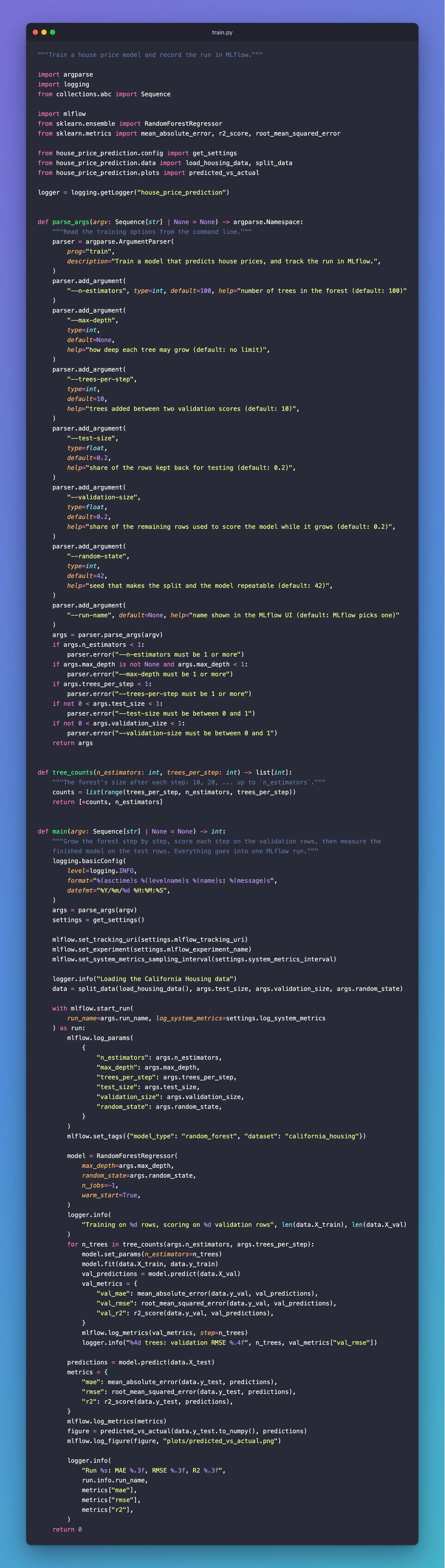
"""Train a house price model and record the run in MLflow."""

import argparse
import logging
from collections.abc import Sequence

import mlflow
from sklearn.ensemble import RandomForestRegressor
from sklearn.metrics import mean_absolute_error, r2_score, root_mean_squared_error

from house_price_prediction.config import get_settings
from house_price_prediction.data import load_housing_data, split_data
from house_price_prediction.plots import predicted_vs_actual

logger = logging.getLogger("house_price_prediction")


def parse_args(argv: Sequence[str] | None = None) -> argparse.Namespace:
    """Read the training options from the command line."""
    parser = argparse.ArgumentParser(
        prog="train",
        description="Train a model that predicts house prices, and track the run in MLflow.",
    )
    parser.add_argument(
        "--n-estimators", type=int, default=100, help="number of trees in the forest (default: 100)"
    )
    parser.add_argument(
        "--max-depth",
        type=int,
        default=None,
        help="how deep each tree may grow (default: no limit)",
    )
    parser.add_argument(
        "--trees-per-step",
        type=int,
        default=10,
        help="trees added between two validation scores (default: 10)",
    )
    parser.add_argument(
        "--test-size",
        type=float,
        default=0.2,
        help="share of the rows kept back for testing (default: 0.2)",
    )
    parser.add_argument(
        "--validation-size",
        type=float,
        default=0.2,
        help="share of the remaining rows used to score the model while it grows (default: 0.2)",
    )
    parser.add_argument(
        "--random-state",
        type=int,
        default=42,
        help="seed that makes the split and the model repeatable (default: 42)",
    )
    parser.add_argument(
        "--run-name", default=None, help="name shown in the MLflow UI (default: MLflow picks one)"
    )
    args = parser.parse_args(argv)
    if args.n_estimators < 1:
        parser.error("--n-estimators must be 1 or more")
    if args.max_depth is not None and args.max_depth < 1:
        parser.error("--max-depth must be 1 or more")
    if args.trees_per_step < 1:
        parser.error("--trees-per-step must be 1 or more")
    if not 0 < args.test_size < 1:
        parser.error("--test-size must be between 0 and 1")
    if not 0 < args.validation_size < 1:
        parser.error("--validation-size must be between 0 and 1")
    return args


def tree_counts(n_estimators: int, trees_per_step: int) -> list[int]:
    """The forest's size after each step: 10, 20, ... up to `n_estimators`."""
    counts = list(range(trees_per_step, n_estimators, trees_per_step))
    return [*counts, n_estimators]


def main(argv: Sequence[str] | None = None) -> int:
    """Grow the forest step by step, score each step on the validation rows, then measure the
    finished model on the test rows. Everything goes into one MLflow run."""
    logging.basicConfig(
        level=logging.INFO,
        format="%(asctime)s %(levelname)s %(name)s: %(message)s",
        datefmt="%Y/%m/%d %H:%M:%S",
    )
    args = parse_args(argv)
    settings = get_settings()

    mlflow.set_tracking_uri(settings.mlflow_tracking_uri)
    mlflow.set_experiment(settings.mlflow_experiment_name)
    mlflow.set_system_metrics_sampling_interval(settings.system_metrics_interval)

    logger.info("Loading the California Housing data")
    data = split_data(load_housing_data(), args.test_size, args.validation_size, args.random_state)

    with mlflow.start_run(
        run_name=args.run_name, log_system_metrics=settings.log_system_metrics
    ) as run:
        mlflow.log_params(
            {
                "n_estimators": args.n_estimators,
                "max_depth": args.max_depth,
                "trees_per_step": args.trees_per_step,
                "test_size": args.test_size,
                "validation_size": args.validation_size,
                "random_state": args.random_state,
            }
        )
        mlflow.set_tags({"model_type": "random_forest", "dataset": "california_housing"})

        model = RandomForestRegressor(
            max_depth=args.max_depth,
            random_state=args.random_state,
            n_jobs=-1,
            warm_start=True,
        )
        logger.info(
            "Training on %d rows, scoring on %d validation rows", len(data.X_train), len(data.X_val)
        )
        for n_trees in tree_counts(args.n_estimators, args.trees_per_step):
            model.set_params(n_estimators=n_trees)
            model.fit(data.X_train, data.y_train)
            val_predictions = model.predict(data.X_val)
            val_metrics = {
                "val_mae": mean_absolute_error(data.y_val, val_predictions),
                "val_rmse": root_mean_squared_error(data.y_val, val_predictions),
                "val_r2": r2_score(data.y_val, val_predictions),
            }
            mlflow.log_metrics(val_metrics, step=n_trees)
            logger.info("%4d trees: validation RMSE %.4f", n_trees, val_metrics["val_rmse"])

        predictions = model.predict(data.X_test)
        metrics = {
            "mae": mean_absolute_error(data.y_test, predictions),
            "rmse": root_mean_squared_error(data.y_test, predictions),
            "r2": r2_score(data.y_test, predictions),
        }
        mlflow.log_metrics(metrics)
        figure = predicted_vs_actual(data.y_test.to_numpy(), predictions)
        mlflow.log_figure(figure, "plots/predicted_vs_actual.png")

        logger.info(
            "Run %s: MAE %.3f, RMSE %.3f, R2 %.3f",
            run.info.run_name,
            metrics["mae"],
            metrics["rmse"],
            metrics["r2"],
        )
    return 0
Step 5: Add a curve Command
The MLflow UI will draw the curves, but a curve is also data you'll want in code: for a report, a test, or to pick the best number of trees. Create src/house_price_prediction/curve.py and build it in two pieces.
The options: the run's name, and which validation score to show:
"""Show how a run's validation score changed as its forest grew, read back from MLflow."""

import argparse
from collections.abc import Sequence

from mlflow import MlflowClient

from house_price_prediction.config import get_settings

LOWER_IS_BETTER = {"val_mae", "val_rmse"}


def parse_args(argv: Sequence[str] | None = None) -> argparse.Namespace:
    """Read the run's name and the score to show from the command line."""
    parser = argparse.ArgumentParser(
        prog="curve",
        description="Print a run's validation score after each training step, and the best step.",
    )
    parser.add_argument("run_name", help="the run's name, as shown in the MLflow UI")
    parser.add_argument(
        "--metric",
        default="val_rmse",
        choices=["val_rmse", "val_mae", "val_r2"],
        help="the score to show (default: val_rmse)",
    )
    return parser.parse_args(argv)
choices makes argparse refuse anything but the three validation scores.
Find the run and read its history. Add below parse_args:
def main(argv: Sequence[str] | None = None) -> int:
    """Find the newest run with the given name and print its metric history, step by step."""
    args = parse_args(argv)
    settings = get_settings()
    client = MlflowClient(tracking_uri=settings.mlflow_tracking_uri)

    experiment = client.get_experiment_by_name(settings.mlflow_experiment_name)
    if experiment is None:
        print(f"No experiment called {settings.mlflow_experiment_name!r}")
        return 1
    runs = client.search_runs([experiment.experiment_id], order_by=["attributes.start_time DESC"])
    run = next((r for r in runs if r.info.run_name == args.run_name), None)
    if run is None:
        print(f"No run called {args.run_name!r} in {experiment.name!r}")
        return 1

    history = sorted(client.get_metric_history(run.info.run_id, args.metric), key=lambda m: m.step)
    if not history:
        print(f"Run {args.run_name!r} has no {args.metric!r} history")
        return 1
    for point in history:
        print(f"{point.step:5d} trees  {args.metric} {point.value:.4f}")
    pick = min if args.metric in LOWER_IS_BETTER else max
    best = pick(history, key=lambda m: m.value)
    print(f"Best {args.metric}: {best.value:.4f} at {best.step} trees")
    return 0
MlflowClientis MLflow's lower-level client. It talks to the same tracking server as the training code, read from the same settings.- The runs come newest first, and the first one with the requested name wins. MLflow doesn't require run names to be unique, so a name you reuse finds your latest run.
get_metric_history()returns every value the metric was logged with, each with its step: How to Get the History of a Metric in MLflow. The run's summary, by contrast, keeps only the last value.- The best step is the lowest value for the two errors and the highest for R².
- It returns 1 when the experiment, the run or the history is missing, so a script that calls it can tell that it failed.
The complete file is the two pieces together:
"""Show how a run's validation score changed as its forest grew, read back from MLflow."""

import argparse
from collections.abc import Sequence

from mlflow import MlflowClient

from house_price_prediction.config import get_settings

LOWER_IS_BETTER = {"val_mae", "val_rmse"}


def parse_args(argv: Sequence[str] | None = None) -> argparse.Namespace:
    """Read the run's name and the score to show from the command line."""
    parser = argparse.ArgumentParser(
        prog="curve",
        description="Print a run's validation score after each training step, and the best step.",
    )
    parser.add_argument("run_name", help="the run's name, as shown in the MLflow UI")
    parser.add_argument(
        "--metric",
        default="val_rmse",
        choices=["val_rmse", "val_mae", "val_r2"],
        help="the score to show (default: val_rmse)",
    )
    return parser.parse_args(argv)


def main(argv: Sequence[str] | None = None) -> int:
    """Find the newest run with the given name and print its metric history, step by step."""
    args = parse_args(argv)
    settings = get_settings()
    client = MlflowClient(tracking_uri=settings.mlflow_tracking_uri)

    experiment = client.get_experiment_by_name(settings.mlflow_experiment_name)
    if experiment is None:
        print(f"No experiment called {settings.mlflow_experiment_name!r}")
        return 1
    runs = client.search_runs([experiment.experiment_id], order_by=["attributes.start_time DESC"])
    run = next((r for r in runs if r.info.run_name == args.run_name), None)
    if run is None:
        print(f"No run called {args.run_name!r} in {experiment.name!r}")
        return 1

    history = sorted(client.get_metric_history(run.info.run_id, args.metric), key=lambda m: m.step)
    if not history:
        print(f"Run {args.run_name!r} has no {args.metric!r} history")
        return 1
    for point in history:
        print(f"{point.step:5d} trees  {args.metric} {point.value:.4f}")
    pick = min if args.metric in LOWER_IS_BETTER else max
    best = pick(history, key=lambda m: m.value)
    print(f"Best {args.metric}: {best.value:.4f} at {best.step} trees")
    return 0
Register the command. In pyproject.toml, add a curve line to [project.scripts], below train:
[project.scripts]
train = "house_price_prediction.train:main"
curve = "house_price_prediction.curve:main"
Step 6: Add psutil
MLflow reads the computer's CPU and memory use through psutil, but doesn't install it for you. Its documentation says: "We explicitly don't include psutil in MLflow's dependencies". Add it to the project:
uv add psutil
Resolved 93 packages in 2.11s
      Built house-price-prediction @ file:///Users/you/source/dewiride-house-price-prediction
Prepared 1 package in 7ms
Uninstalled 1 package in 1ms
Installed 2 packages in 2ms
 ~ house-price-prediction==0.1.0 (from file:///Users/you/source/dewiride-house-price-prediction)
 + psutil==7.2.2
+ psutil==7.2.2: the new package, now listed inpyproject.tomland locked inuv.lock.~ house-price-prediction: uv rebuilt your own project, becausepyproject.tomlchanged. That's what makes the newcurvecommand available.
Without psutil, a run with system metrics on doesn't even start: How to Check CPU and Memory Usage in Python with psutil introduces the package itself.
Step 7: Train Three Forests
Train the default forest first, 100 trees in steps of 10:
uv run train --run-name curve-100-trees
2026/11/18 10:48:29 INFO house_price_prediction: Loading the California Housing data
2026/11/18 10:48:30 INFO mlflow.system_metrics.system_metrics_monitor: Skip logging GPU metrics. Set logger level to DEBUG for more details.
2026/11/18 10:48:30 INFO mlflow.system_metrics.system_metrics_monitor: Started monitoring system metrics.
2026/11/18 10:48:30 INFO house_price_prediction: Training on 13209 rows, scoring on 3303 validation rows
2026/11/18 10:48:30 INFO house_price_prediction:   10 trees: validation RMSE 0.5490
2026/11/18 10:48:30 INFO house_price_prediction:   20 trees: validation RMSE 0.5417
2026/11/18 10:48:30 INFO house_price_prediction:   30 trees: validation RMSE 0.5363
2026/11/18 10:48:30 INFO house_price_prediction:   40 trees: validation RMSE 0.5320
2026/11/18 10:48:30 INFO house_price_prediction:   50 trees: validation RMSE 0.5308
2026/11/18 10:48:30 INFO house_price_prediction:   60 trees: validation RMSE 0.5300
2026/11/18 10:48:30 INFO house_price_prediction:   70 trees: validation RMSE 0.5301
2026/11/18 10:48:31 INFO house_price_prediction:   80 trees: validation RMSE 0.5287
2026/11/18 10:48:31 INFO house_price_prediction:   90 trees: validation RMSE 0.5283
2026/11/18 10:48:31 INFO house_price_prediction:  100 trees: validation RMSE 0.5276
2026/11/18 10:48:31 INFO house_price_prediction: Run curve-100-trees: MAE 0.337, RMSE 0.516, R2 0.797
🏃 View run curve-100-trees at: http://127.0.0.1:8080/#/experiments/1/runs/3f7155effd274ec884c35e62025969a8
🧪 View experiment at: http://127.0.0.1:8080/#/experiments/1
2026/11/18 10:48:31 INFO mlflow.system_metrics.system_metrics_monitor: Stopping system metrics monitoring...
2026/11/18 10:48:31 INFO mlflow.system_metrics.system_metrics_monitor: Successfully terminated system metrics monitoring!
Line by line:
Skip logging GPU metrics: MLflow couldn't start a monitor for an NVIDIA or AMD graphics card. That's expected on a Mac; elsewhere, GPU monitoring needs extra packages.Started monitoring system metrics: the run's monitor is sampling the computer every second.Training on 13209 rows, scoring on 3303 validation rows: the three-way split from Step 2.- One line per stage. The validation error falls fast at first, from 0.5490 at 10 trees to 0.5308 at 50, then barely moves: 0.5276 at 100.
- The test scores: MAE 0.337, RMSE 0.516, R² 0.797. Part 1's 100-tree forest scored 0.328, 0.506 and 0.804 on the same test rows. The difference is the data it learned from: 13,209 rows instead of 16,512, because the validation rows came out of the training rows. That's the price of a validation set.
Stopping system metrics monitoring: the run ended, and its monitor with it.
Now two more forests: 300 trees, 20 at a time, and a forest whose trees may only grow 8 levels deep:
uv run train --n-estimators 300 --trees-per-step 20 --run-name curve-300-trees
uv run train --max-depth 8 --run-name curve-depth-8
2026/11/18 10:49:48 INFO house_price_prediction: Loading the California Housing data
2026/11/18 10:49:48 INFO mlflow.system_metrics.system_metrics_monitor: Skip logging GPU metrics. Set logger level to DEBUG for more details.
2026/11/18 10:49:48 INFO mlflow.system_metrics.system_metrics_monitor: Started monitoring system metrics.
2026/11/18 10:49:48 INFO house_price_prediction: Training on 13209 rows, scoring on 3303 validation rows
2026/11/18 10:49:49 INFO house_price_prediction:   20 trees: validation RMSE 0.5417
2026/11/18 10:49:49 INFO house_price_prediction:   40 trees: validation RMSE 0.5320
2026/11/18 10:49:49 INFO house_price_prediction:   60 trees: validation RMSE 0.5300
2026/11/18 10:49:49 INFO house_price_prediction:   80 trees: validation RMSE 0.5287
2026/11/18 10:49:49 INFO house_price_prediction:  100 trees: validation RMSE 0.5276
2026/11/18 10:49:50 INFO house_price_prediction:  120 trees: validation RMSE 0.5266
2026/11/18 10:49:50 INFO house_price_prediction:  140 trees: validation RMSE 0.5261
2026/11/18 10:49:50 INFO house_price_prediction:  160 trees: validation RMSE 0.5254
2026/11/18 10:49:50 INFO house_price_prediction:  180 trees: validation RMSE 0.5254
2026/11/18 10:49:50 INFO house_price_prediction:  200 trees: validation RMSE 0.5254
2026/11/18 10:49:51 INFO house_price_prediction:  220 trees: validation RMSE 0.5250
2026/11/18 10:49:51 INFO house_price_prediction:  240 trees: validation RMSE 0.5253
2026/11/18 10:49:51 INFO house_price_prediction:  260 trees: validation RMSE 0.5248
2026/11/18 10:49:51 INFO house_price_prediction:  280 trees: validation RMSE 0.5244
2026/11/18 10:49:52 INFO house_price_prediction:  300 trees: validation RMSE 0.5243
2026/11/18 10:49:52 INFO house_price_prediction: Run curve-300-trees: MAE 0.334, RMSE 0.512, R2 0.800
🏃 View run curve-300-trees at: http://127.0.0.1:8080/#/experiments/1/runs/66d6ec9ec6ad4f10bb337e57549c3d4f
🧪 View experiment at: http://127.0.0.1:8080/#/experiments/1
2026/11/18 10:49:52 INFO mlflow.system_metrics.system_metrics_monitor: Stopping system metrics monitoring...
2026/11/18 10:49:52 INFO mlflow.system_metrics.system_metrics_monitor: Successfully terminated system metrics monitoring!
2026/11/18 10:49:56 INFO house_price_prediction: Loading the California Housing data
2026/11/18 10:49:56 INFO mlflow.system_metrics.system_metrics_monitor: Skip logging GPU metrics. Set logger level to DEBUG for more details.
2026/11/18 10:49:56 INFO mlflow.system_metrics.system_metrics_monitor: Started monitoring system metrics.
2026/11/18 10:49:56 INFO house_price_prediction: Training on 13209 rows, scoring on 3303 validation rows
2026/11/18 10:49:56 INFO house_price_prediction:   10 trees: validation RMSE 0.5939
2026/11/18 10:49:56 INFO house_price_prediction:   20 trees: validation RMSE 0.5922
2026/11/18 10:49:56 INFO house_price_prediction:   30 trees: validation RMSE 0.5888
2026/11/18 10:49:56 INFO house_price_prediction:   40 trees: validation RMSE 0.5875
2026/11/18 10:49:56 INFO house_price_prediction:   50 trees: validation RMSE 0.5875
2026/11/18 10:49:56 INFO house_price_prediction:   60 trees: validation RMSE 0.5867
2026/11/18 10:49:56 INFO house_price_prediction:   70 trees: validation RMSE 0.5872
2026/11/18 10:49:56 INFO house_price_prediction:   80 trees: validation RMSE 0.5862
2026/11/18 10:49:57 INFO house_price_prediction:   90 trees: validation RMSE 0.5861
2026/11/18 10:49:57 INFO house_price_prediction:  100 trees: validation RMSE 0.5857
2026/11/18 10:49:57 INFO house_price_prediction: Run curve-depth-8: MAE 0.403, RMSE 0.586, R2 0.738
🏃 View run curve-depth-8 at: http://127.0.0.1:8080/#/experiments/1/runs/60a6a374e9724a86bd4a3b401de03142
🧪 View experiment at: http://127.0.0.1:8080/#/experiments/1
2026/11/18 10:49:57 INFO mlflow.system_metrics.system_metrics_monitor: Stopping system metrics monitoring...
2026/11/18 10:49:57 INFO mlflow.system_metrics.system_metrics_monitor: Successfully terminated system metrics monitoring!
- The 300-tree forest matches the 100-tree one stage for stage, 0.5417 at 20 trees and 0.5276 at 100, because both start from the same
random_stateand grow the same trees in the same order. The next 200 trees take the error from 0.5276 to 0.5243. - The depth-8 forest is worse at every stage, and more trees hardly help: 0.5939 at 10 trees, 0.5857 at 100. Shallow trees can't capture enough detail, however many there are.
Your times and run IDs will differ.
Step 8: See One Run's Curves
Open the curve-300-trees link from the output and click Model metrics:
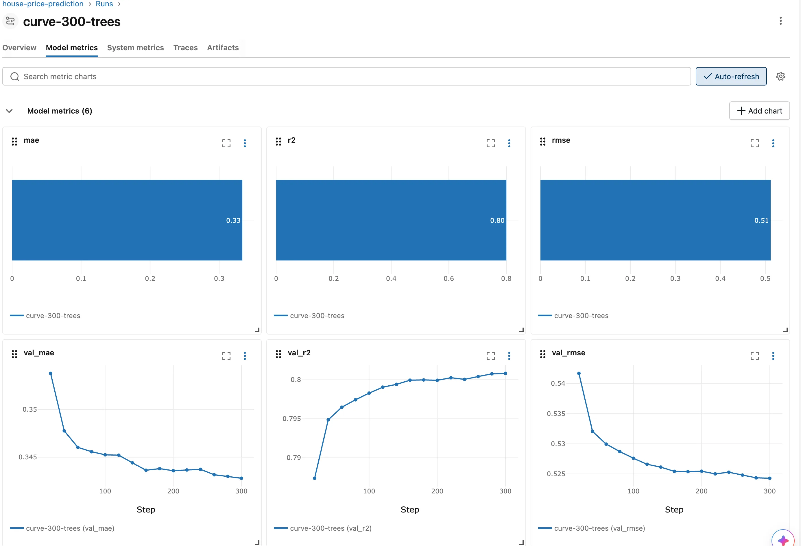
- The three
val_metrics are lines, with Step, the number of trees, along the bottom. MLflow drew a line because each was logged at 15 steps. mae,r2andrmseare bars. They were logged once, so there's nothing to draw a line through.- The shape is the lesson: the error drops steeply over the first 60 trees, then flattens. Most of what a forest learns, it learns early.
Step 9: Compare the Curves of Three Runs
Open the house-price-prediction experiment and click the chart icon above the runs table, as in Part 1. Part 1's four runs have no curves, so hide them from the charts: click the eye icon next to each of their names. The three new runs remain:
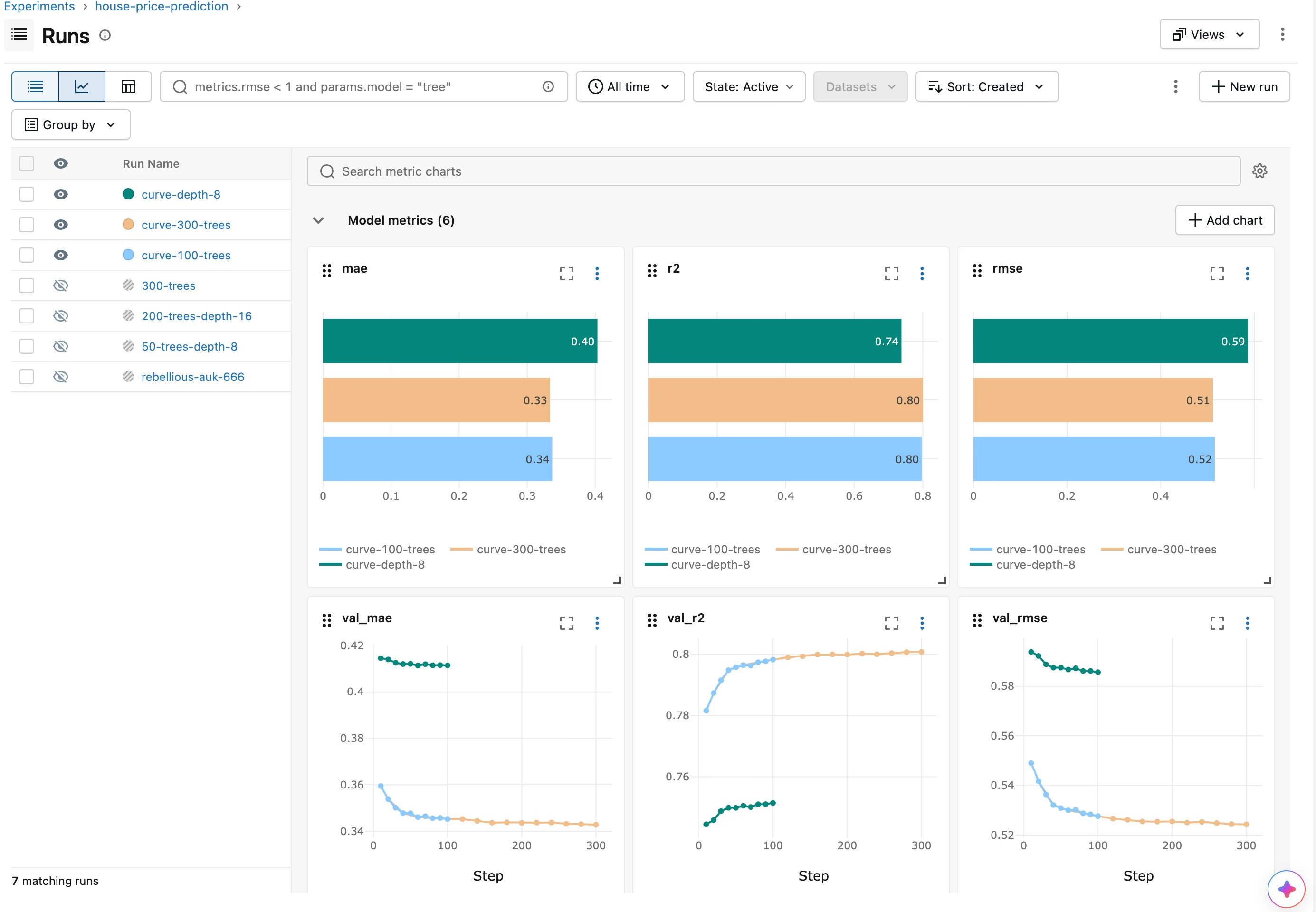
What the curves say, without a single extra run:
- Blue and orange overlap up to 100 trees. They're the same forest, scored every 10 trees in one run and every 20 in the other.
- Orange shows what trees 100 to 300 add: almost nothing, a 0.6% lower error for three times the trees.
- Green sits apart. Limiting the depth costs more than any number of trees can win back.
So 100 unlimited trees, Part 1's default, stays a sound choice, and now the curves show why. The X-axis can also show time instead of steps: How to Change the X-Axis of a Metric Chart in the MLflow UI.
Step 10: Read a Curve from Python
The same curve, from the command you added in Step 5:
uv run curve curve-300-trees
   20 trees  val_rmse 0.5417
   40 trees  val_rmse 0.5320
   60 trees  val_rmse 0.5300
   80 trees  val_rmse 0.5287
  100 trees  val_rmse 0.5276
  120 trees  val_rmse 0.5266
  140 trees  val_rmse 0.5261
  160 trees  val_rmse 0.5254
  180 trees  val_rmse 0.5254
  200 trees  val_rmse 0.5254
  220 trees  val_rmse 0.5250
  240 trees  val_rmse 0.5253
  260 trees  val_rmse 0.5248
  280 trees  val_rmse 0.5244
  300 trees  val_rmse 0.5243
Best val_rmse: 0.5243 at 300 trees
Every value the run logged came back, in step order. The best is at 300 trees, but only by a little, which is why the curve matters more than the single best number. Ask for R² instead, on the depth-8 run:
uv run curve curve-depth-8 --metric val_r2
   10 trees  val_r2 0.7444
   20 trees  val_r2 0.7458
   30 trees  val_r2 0.7488
   40 trees  val_r2 0.7499
   50 trees  val_r2 0.7499
   60 trees  val_r2 0.7505
   70 trees  val_r2 0.7501
   80 trees  val_r2 0.7510
   90 trees  val_r2 0.7510
  100 trees  val_r2 0.7514
Best val_r2: 0.7514 at 100 trees
For R², higher is better, so the command picked the highest value. The shallow forest never explains more than about 75% of the variation.
Step 11: See the System Metrics
Open the curve-300-trees run again and click System metrics:
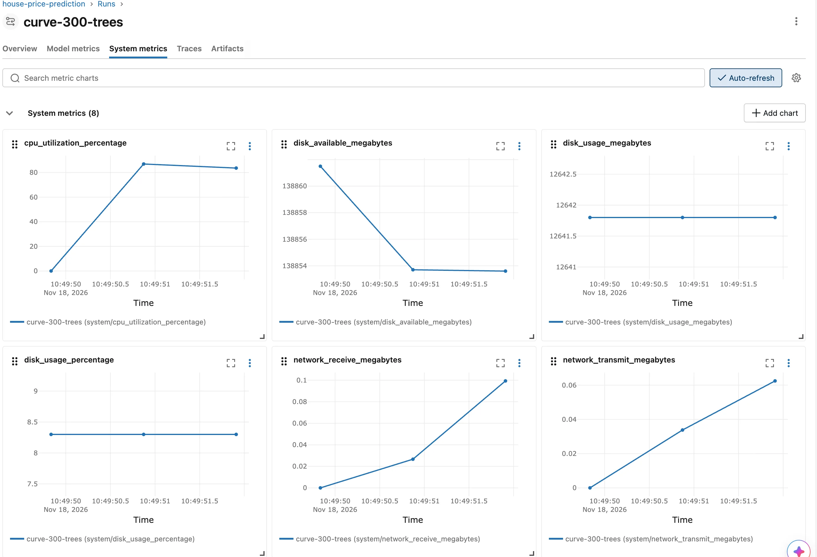
- Eight charts, with time along the bottom, one for each
system/metric MLflow recorded. - CPU went from 0 to about 87%. The first CPU sample of every run is
0.0: psutil's first reading in each new thread is "a meaningless 0.0 value", and each run's monitor is a new thread. After that, the forest kept the processor busy on all cores, becausen_jobs=-1uses them all. The figure covers the whole computer, not only this program. - Three samples, for a run that lasted 3.7 seconds at one sample per second. The monitor logs a sample only when a whole interval has passed and the run is still going, so the sample taken in a run's last second is never logged.
The curve-depth-8 run lasted 1.0 second on this computer, and its System metrics tab says System metrics (0) and "No charts in this section": it ended before its first sample could be logged. Fixed: "No charts in this section" on the MLflow System Metrics Tab walks through the cause. To record its system metrics, train it again with a sample every 0.2 seconds. The new setting from Step 3 changes the interval for this one command:
- macOS / Linux
- Windows (PowerShell)
HOUSE_PRICES_SYSTEM_METRICS_INTERVAL=0.2 uv run train --max-depth 8 --run-name curve-depth-8-sampled
$env:HOUSE_PRICES_SYSTEM_METRICS_INTERVAL = "0.2"
uv run train --max-depth 8 --run-name curve-depth-8-sampled
Remove-Item Env:HOUSE_PRICES_SYSTEM_METRICS_INTERVAL
2026/11/18 10:58:40 INFO house_price_prediction: Loading the California Housing data
2026/11/18 10:58:40 INFO mlflow.system_metrics.system_metrics_monitor: Skip logging GPU metrics. Set logger level to DEBUG for more details.
2026/11/18 10:58:40 INFO mlflow.system_metrics.system_metrics_monitor: Started monitoring system metrics.
2026/11/18 10:58:40 INFO house_price_prediction: Training on 13209 rows, scoring on 3303 validation rows
2026/11/18 10:58:40 INFO house_price_prediction:   10 trees: validation RMSE 0.5939
2026/11/18 10:58:40 INFO house_price_prediction:   20 trees: validation RMSE 0.5922
2026/11/18 10:58:40 INFO house_price_prediction:   30 trees: validation RMSE 0.5888
2026/11/18 10:58:40 INFO house_price_prediction:   40 trees: validation RMSE 0.5875
2026/11/18 10:58:40 INFO house_price_prediction:   50 trees: validation RMSE 0.5875
2026/11/18 10:58:40 INFO house_price_prediction:   60 trees: validation RMSE 0.5867
2026/11/18 10:58:40 INFO house_price_prediction:   70 trees: validation RMSE 0.5872
2026/11/18 10:58:40 INFO house_price_prediction:   80 trees: validation RMSE 0.5862
2026/11/18 10:58:40 INFO house_price_prediction:   90 trees: validation RMSE 0.5861
2026/11/18 10:58:41 INFO house_price_prediction:  100 trees: validation RMSE 0.5857
2026/11/18 10:58:41 INFO house_price_prediction: Run curve-depth-8-sampled: MAE 0.403, RMSE 0.586, R2 0.738
🏃 View run curve-depth-8-sampled at: http://127.0.0.1:8080/#/experiments/1/runs/a5c92ce28557481999f160318456da7a
🧪 View experiment at: http://127.0.0.1:8080/#/experiments/1
2026/11/18 10:58:41 INFO mlflow.system_metrics.system_metrics_monitor: Stopping system metrics monitoring...
2026/11/18 10:58:41 INFO mlflow.system_metrics.system_metrics_monitor: Successfully terminated system metrics monitoring!
The same scores as curve-depth-8, and this time the run's System metrics tab has all eight charts, five samples each:
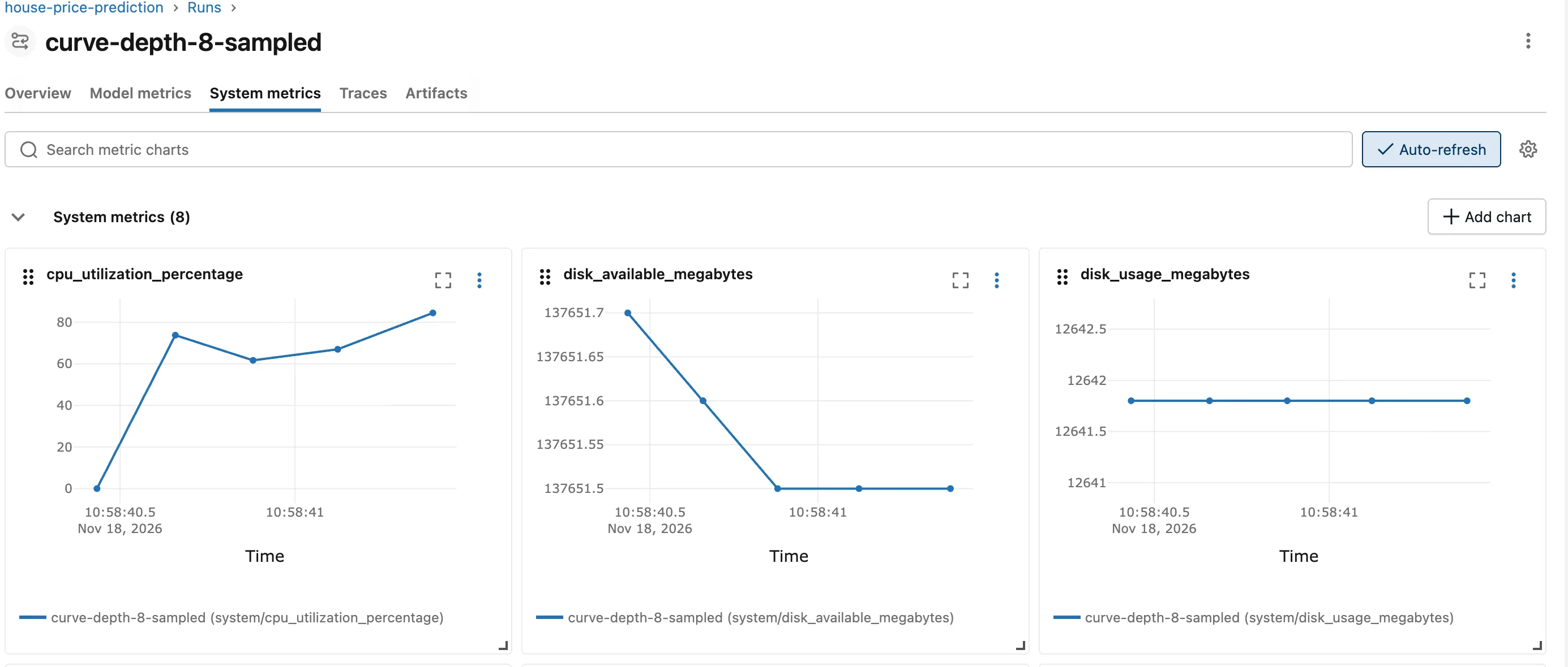
How long a run takes depends on your computer. If your curve-depth-8 run lasted longer than a second, its tab has charts already.
Step 12: Save Your Work with Git
See what changed since Part 1's commit:
git status --short --untracked-files=all
 M .env.example
 M pyproject.toml
 M src/house_price_prediction/config.py
 M src/house_price_prediction/data.py
 M src/house_price_prediction/train.py
 M uv.lock
?? src/house_price_prediction/curve.py
M marks a changed file and ?? a new one: the five files you edited, the lock file that uv add updated, and the new curve.py. How to See What Changed in a Git Repository Before You Commit explains the codes. Commit them:
git add .
git commit -m "Log validation curves and system metrics"
[master e6b8df4] Log validation curves and system metrics
 7 files changed, 151 insertions(+), 14 deletions(-)
 create mode 100644 src/house_price_prediction/curve.py
Your commit ID will differ.
Your Folders Now Look Like This
source/
├── mlflow-server/
│   ├── .venv/
│   ├── mlartifacts/
│   ├── mlflow.db
│   ├── pyproject.toml
│   └── uv.lock
└── dewiride-house-price-prediction/
    ├── .venv/
    ├── src/
    │   └── house_price_prediction/
    │       ├── __init__.py
    │       ├── config.py
    │       ├── curve.py
    │       ├── data.py
    │       ├── plots.py
    │       └── train.py
    ├── .env
    ├── .env.example
    ├── .gitignore
    ├── .python-version
    ├── README.md
    ├── pyproject.toml
    └── uv.lock
The step metrics and system metrics went where every metric goes: into the metrics table of mlflow-server/mlflow.db, one row per value, each with its step.
Stop the Server When You're Done
Go to the first terminal and press Ctrl+C. Your runs stay in mlflow.db and mlartifacts/, and uv run mlflow server --port 8080 in the mlflow-server folder brings them back.
Keep both folders for Part 3. If you ever want to remove everything the series created, stop the server first, then delete the mlflow-server and dewiride-house-price-prediction folders, and the scikit_learn_data folder in your home folder.
Common Mistakes
| Mistake | What happens | Do this instead |
|---|---|---|
| Choosing the number of trees by the test score | The test score stops being a fair check on unseen data | Watch a validation set, and score the test set once at the end |
Logging a value at every stage without step= | Every value is stored at step 0, so there's no curve to read | Pass step=, such as the number of trees or the epoch |
Leaving out warm_start=True | Each stage grows a whole new forest, so training takes far longer | Set warm_start=True and raise n_estimators between fits |
Setting the sampling interval after start_run | The run's monitor keeps the interval it started with | Call mlflow.set_system_metrics_sampling_interval() first |
| Keeping MLflow's 10-second default for runs of a few seconds | The System metrics tab stays empty | Sample more often than your shortest run lasts |
| Comparing Part 2's test scores with Part 1's and blaming the code | The difference comes from the smaller training set | Compare runs that learned from the same rows |
Troubleshooting
| Symptom | Likely cause | Fix |
|---|---|---|
MlflowException: Failed to start system metrics monitoring as package `psutil` is not installed. | psutil is missing | uv add psutil (Step 6) |
| System metrics (0), "No charts in this section" | The run ended within one sampling interval | A shorter interval: Fixed: "No charts in this section" on the MLflow System Metrics Tab |
No run called 'curve-300' in 'house-price-prediction' | No run has exactly that name | Copy the name from the runs table |
curve: error: argument --metric: invalid choice: 'rmse', maybe you meant 'val_rmse'? | curve only reads the validation scores | Use val_rmse, val_mae or val_r2 |
| Part 1's runs crowd the charts as bars with no curve | They logged each score once | Hide them with the eye icon next to their names |
FAQ
Why not watch the test score while training?
Because then you'd be choosing the model with the test rows, and their score would no longer tell you how the model does on data it has never seen. The validation rows take that role, and the test rows stay untouched until the end.
What can a step be?
Any whole number you choose. MLflow stores it with each value and draws the curve along it. Common choices are the epoch for neural networks, the number of trees for forests and boosting, or simply a counter.
Does logging at every step slow training down?
Each log_metrics call sends one request to the tracking server, here 10 to 15 per run. A loop with thousands of steps can log every tenth or hundredth step instead.
Why does the CPU chart always start at 0?
The first CPU reading in each new thread is 0.0, and every run's monitor is a new thread. Read the chart from its second point. How to Turn On System Metrics Logging in MLflow has the details.
Can I monitor a GPU?
MLflow's documentation lists extra packages for NVIDIA and AMD graphics cards. Without one, MLflow prints Skip logging GPU metrics and records the other eight metrics, as here.
Conclusion
Your forest now grows in stages, and after each stage mlflow.log_metrics(..., step=n_trees) records three validation scores, scored on rows the model never trains on. The MLflow UI turned them into learning curves, which showed that trees beyond 100 add almost nothing and that a depth limit costs more than trees can win back. The curve command read the same curve with get_metric_history(), and system metrics recorded the processor, memory, disk and network for every run long enough to be sampled.
In Part 3 you'll attach whole files and the exact dataset each run used, and search runs from Python.
Additional Resources
- mlflow.log_metrics — MLflow's reference, including
step. - MlflowClient.get_metric_history — reading every value of a metric.
- System Metrics — MLflow's guide to system metrics and their settings.
- RandomForestRegressor — scikit-learn's reference, including
warm_start.
← Previous: Part 1: Install MLflow and Track Your First Experiment
Next → Part 3: Log Artifacts and Datasets (coming soon)
