How to Plot Predicted vs Actual Values with Matplotlib

A single error score tells you how much a regression model misses on average. A predicted vs actual chart shows where it misses: which values it gets right, which it underestimates, and where the data itself is odd. This guide draws the chart with Matplotlib, saves it as a PNG, and reads a real one from a scikit-learn model.
Syntax
from matplotlib.figure import Figure

figure = Figure(figsize=(<width>, <height>))
axes = figure.subplots()
axes.scatter(<actual values>, <predicted values>)
axes.plot([<low>, <high>], [<low>, <high>], linestyle="--")
figure.savefig("<file name>.png")
| Part | What it means |
|---|---|
Figure(figsize=(width, height)) | A new, empty chart, width by height inches |
figure.subplots() | Adds one set of axes to draw on |
axes.scatter(actual, predicted) | One dot per row: the real value across, the prediction up |
axes.plot([low, high], [low, high]) | The diagonal where the prediction equals the real value. A dot on it is a perfect prediction |
figure.savefig(path) | Saves the chart to a file. The extension picks the format |
Prerequisites
- A uv project with Matplotlib and scikit-learn, for example after
uv add matplotlib scikit-learn. See How to Add a Package to a Python Project with uv. - Predictions to plot. This guide trains the random forest from How to Train a Random Forest Regression Model with scikit-learn.
Step 1: Write the Plot Function
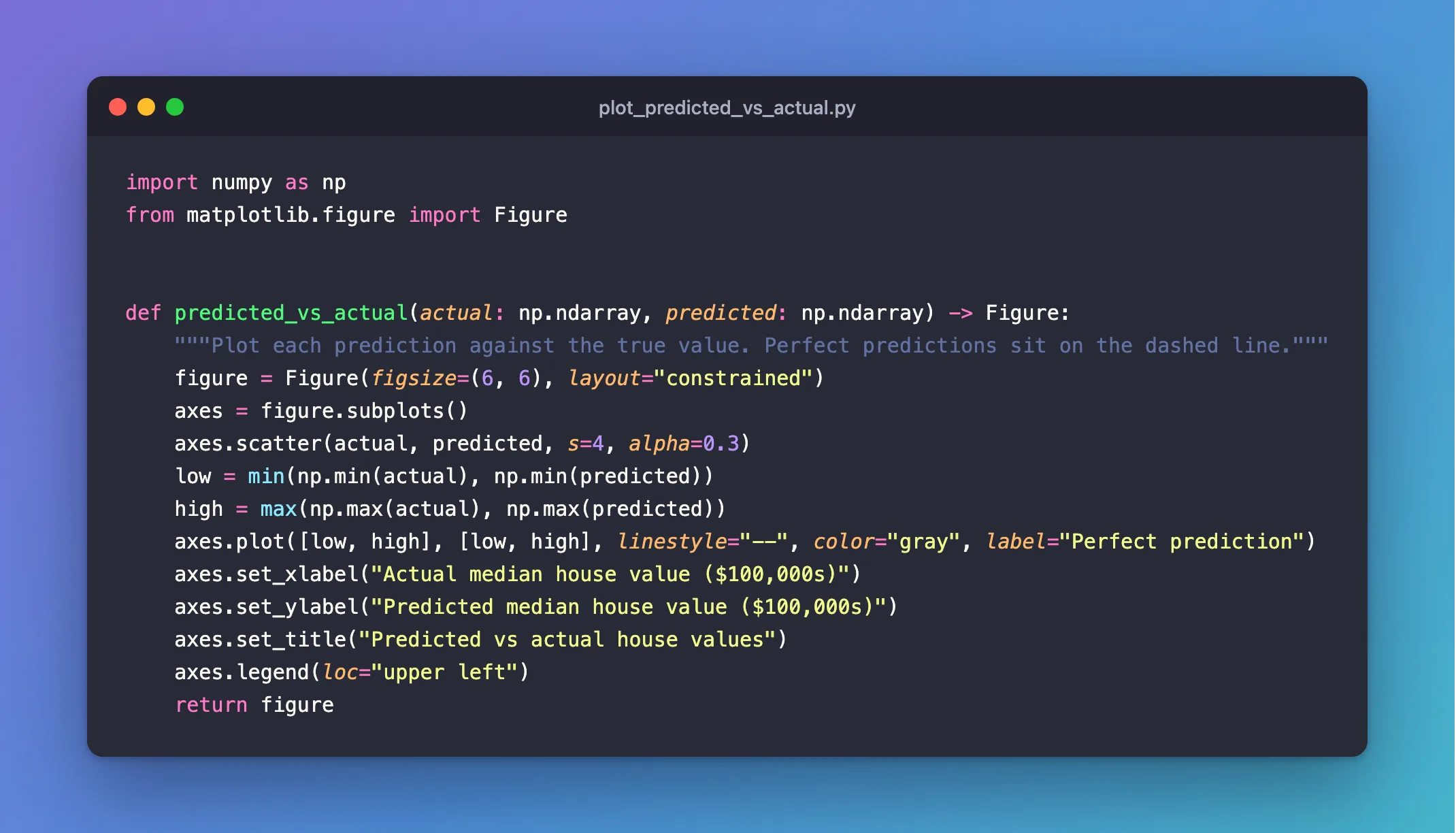
import numpy as np
from matplotlib.figure import Figure


def predicted_vs_actual(actual: np.ndarray, predicted: np.ndarray) -> Figure:
    """Plot each prediction against the true value. Perfect predictions sit on the dashed line."""
    figure = Figure(figsize=(6, 6), layout="constrained")
    axes = figure.subplots()
    axes.scatter(actual, predicted, s=4, alpha=0.3)
    low = min(np.min(actual), np.min(predicted))
    high = max(np.max(actual), np.max(predicted))
    axes.plot([low, high], [low, high], linestyle="--", color="gray", label="Perfect prediction")
    axes.set_xlabel("Actual median house value ($100,000s)")
    axes.set_ylabel("Predicted median house value ($100,000s)")
    axes.set_title("Predicted vs actual house values")
    axes.legend(loc="upper left")
    return figure
| Line | What it does |
|---|---|
Figure(figsize=(6, 6), layout="constrained") | A square figure, 6 by 6 inches. A square makes the diagonal a true 45° line. constrained keeps the labels from being cut off |
axes.scatter(..., s=4, alpha=0.3) | One small, semi-transparent dot per prediction, so dense areas look darker |
axes.plot([low, high], [low, high], ...) | The dashed diagonal where predicted equals actual |
set_xlabel, set_ylabel, set_title | Labels with units, so the chart makes sense on its own |
Why Figure and not pyplot? matplotlib.pyplot keeps every figure it creates in memory until you close it, and needs a display backend. Matplotlib's own documentation says: "When using Matplotlib in a web server it is strongly recommended to not use pyplot (pyplot maintains references to the opened figures to make show work, but this will cause memory leaks unless the figures are properly closed)." A Figure built directly is an ordinary object that Python frees when you're done, so it's safe in scripts, servers and training jobs.
Step 2: Train a Model and Save the Chart
Add below the function:
from sklearn.datasets import fetch_california_housing
from sklearn.ensemble import RandomForestRegressor
from sklearn.model_selection import train_test_split

frame = fetch_california_housing(as_frame=True).frame
X, y = frame.drop(columns="MedHouseVal"), frame["MedHouseVal"]
X_train, X_test, y_train, y_test = train_test_split(X, y, test_size=0.2, random_state=42)
model = RandomForestRegressor(n_estimators=100, random_state=42, n_jobs=-1).fit(X_train, y_train)

figure = predicted_vs_actual(y_test.to_numpy(), model.predict(X_test))
figure.savefig("predicted_vs_actual.png", dpi=150)
print("Saved predicted_vs_actual.png")
In the complete file, keep all imports together at the top. Run it:
uv run python plot_predicted_vs_actual.py
Saved predicted_vs_actual.png
savefig writes the image; dpi=150 makes it 900 by 900 pixels (6 inches × 150 dots per inch).
Step 3: Read the Chart
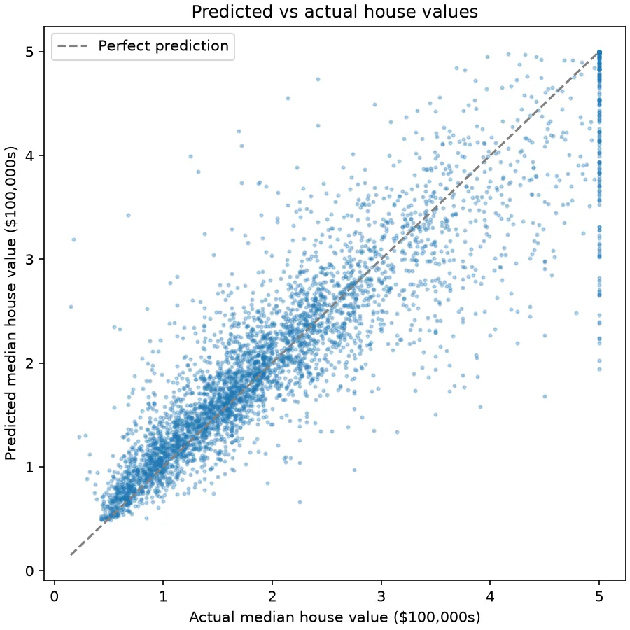
Each dot is one district from the test set: its real value across, the model's guess up.
- Dots on the dashed line are perfect predictions. Most cheap and mid-priced districts sit close to it: the model is good there.
- The cloud widens as values grow. Above about 3 ($300,000) the dots spread further from the line, so errors get bigger for expensive districts.
- Dots below the line are underestimates. At the top right, most dots are under the line: the model tends to guess too low for expensive areas.
- The vertical column at 5.0 is the data, not the model. The dataset caps every district at 5.0 ($500,000), so districts worth far more all share the same "actual" value, while the model's guesses for them range from about 2 to 5.
That last point is something no single score would ever show you.
Common Mistakes
| Mistake | What happens | Do this instead |
|---|---|---|
| Plotting predictions for the training rows | The dots hug the line, because the model has seen those rows: this forest scores R² 0.974 on its training rows against 0.804 on the test rows | Plot the test set |
| A rectangular figure | The diagonal isn't at 45°, so distances to it look skewed | Use a square figsize |
Creating many figures with pyplot in a loop | Memory grows until you call plt.close() | Build a Figure directly, as above |
| No axis labels or units | Nobody can read the chart later | Label both axes with units |
Troubleshooting
| Symptom | Likely cause | Fix |
|---|---|---|
| A solid blob with no detail | Too many large, opaque dots | Lower s and alpha, as in s=4, alpha=0.3 |
| Labels cut off at the edges | The default layout doesn't make room | Use layout="constrained" |
FAQ
Can I log this chart to MLflow instead of saving a file?
Yes. Pass the figure to mlflow.log_figure(): How to Log a Matplotlib Figure to MLflow.
Does this work for classification models?
No, a classifier predicts classes, not numbers. Classifiers use other charts, such as a confusion matrix.
What about the error numbers?
They complement the chart: How to Calculate MAE, RMSE and R² in scikit-learn.
Conclusion
predicted_vs_actual() built a square Figure with one dot per test district and a dashed perfect-prediction line, and savefig wrote it as a PNG. The chart showed what the scores alone couldn't: good predictions for most districts, bigger misses and underestimates for expensive ones, and a column of capped values at $500,000.
Additional Resources
- matplotlib.figure.Figure — the
Figureclass. - Embed in a web application server — Matplotlib's advice on avoiding
pyplotin servers. - Visualizing regression model predictions — scikit-learn's own example of this chart.
