How to Compare Runs with a Parallel Coordinates Plot in the MLflow UI

A table of runs tells you which run won; a parallel coordinates plot shows why. Each run becomes a line that crosses one axis per setting and ends on its score, colored from worst to best, so the settings that lead to good scores stand out at a glance. MLflow draws it on its Compare page. This guide compares six runs of a classifier, with screenshots from MLflow 3.18.0.
Prerequisites
- An MLflow tracking server at
http://127.0.0.1:8080, with its UI open in your browser. MLflow's tracking server guide shows how to start one.
Step 1: Create Runs to Compare
The example scores a k-nearest-neighbors classifier on the iris flowers for every combination of two settings: n_neighbors of 1, 5 or 15, and weights of uniform or distance, six runs in all. Create parallel_runs.py:
import mlflow
from sklearn.datasets import load_iris
from sklearn.model_selection import cross_val_score
from sklearn.neighbors import KNeighborsClassifier

mlflow.set_tracking_uri("http://127.0.0.1:8080")
mlflow.set_experiment("parallel-demo")

X, y = load_iris(return_X_y=True)

for k in [1, 5, 15]:
    for weights in ["uniform", "distance"]:
        with mlflow.start_run(run_name=f"k{k}-{weights}"):
            model = KNeighborsClassifier(n_neighbors=k, weights=weights)
            mlflow.log_params({"n_neighbors": k, "weights": weights})
            mlflow.log_metric("accuracy", cross_val_score(model, X, y, cv=5).mean())
uv run python parallel_runs.py
It prints a View run link for each of the six runs.
Step 2: Select the Runs and Click Compare
Open the experiment parallel-demo. Tick the box in the table's header to select every run, or tick the runs one by one. A row of buttons replaces the search bar:
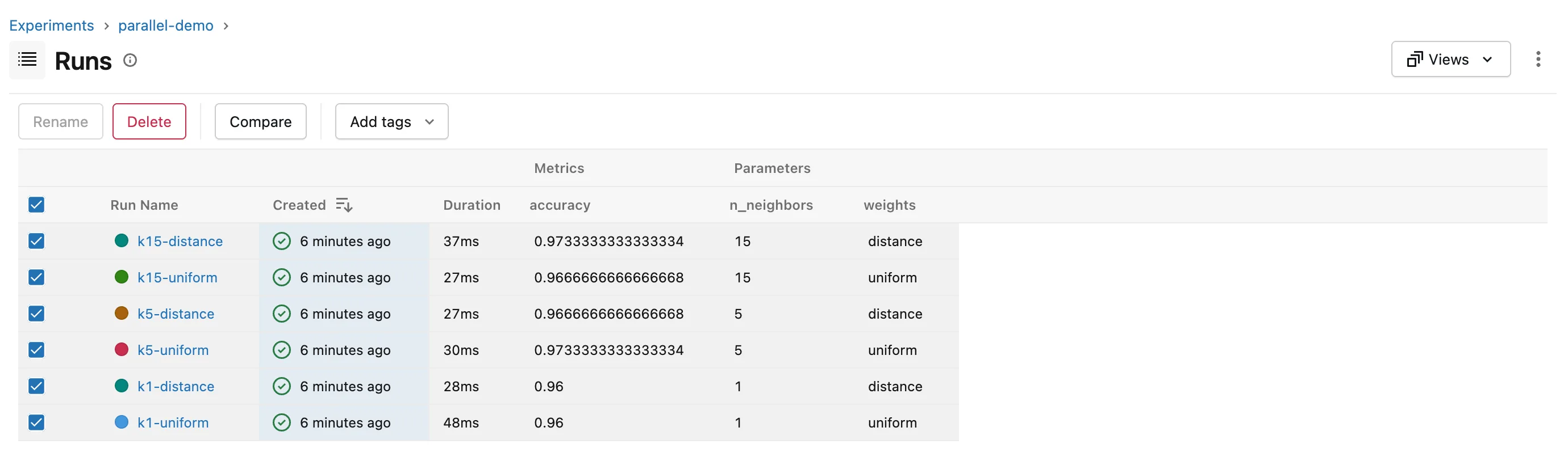
Click Compare.
Step 3: Read the Parallel Coordinates Plot
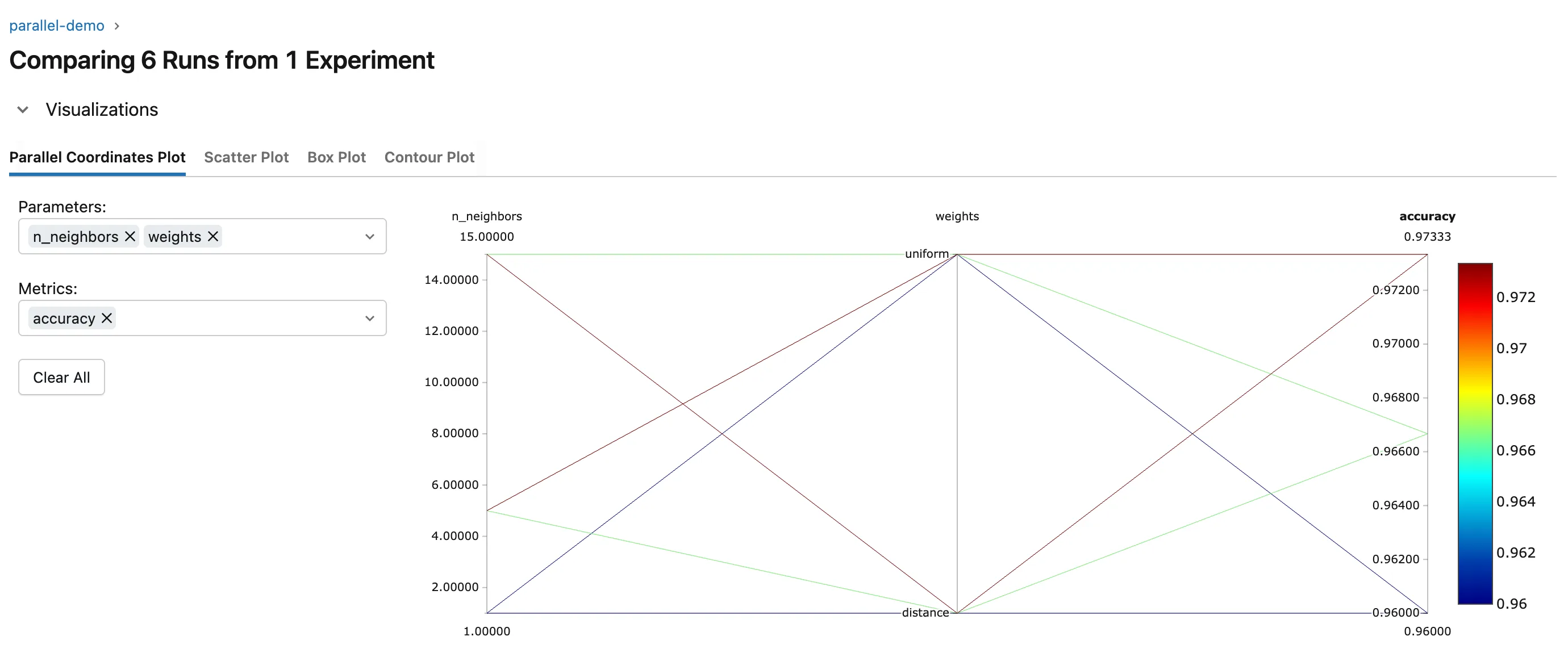
The Compare page opens on Parallel Coordinates Plot. It picked the runs' parameters and their only metric by itself; choose others in the Parameters and Metrics boxes on the left:
How to read it:
- One line per run, from its
n_neighbors, through itsweights, to itsaccuracy. - The color comes from the last axis: dark red for the best accuracy, blue for the worst.
- Follow the red lines back to see which settings they share. Here both top runs, 0.9733, came from 5 or 15 neighbors, and the two blue lines, the lowest at 0.96, from a single neighbor: one neighbor is the weak setting, and
weightsmattered less.
With only two settings the table could tell you as much; with more settings and more runs, as in a hyperparameter search, the plot shows patterns a table hides.
Common Mistakes
| Mistake | What happens | Do this instead |
|---|---|---|
| Choosing a timing metric | The plot colors runs by speed, not quality | Pick the score in Metrics |
Troubleshooting
| Symptom | Likely cause | Fix |
|---|---|---|
| No Compare button | No runs are ticked | Tick the runs you want to compare |
| An axis you need is missing | It isn't in the Parameters or Metrics box | Add it there |
FAQ
Can I compare the children of a hyperparameter search?
Yes: unfold the parent, tick its children, and click Compare. How to Log a GridSearchCV Search in MLflow with Parent and Child Runs creates such children.
What are the other tabs?
Scatter Plot, Box Plot and Contour Plot show the same runs in other ways, such as one setting against the metric. How to Compare Runs in the MLflow UI covers the Compare page.
Conclusion
Ticking six runs and clicking Compare drew a line per run from n_neighbors and weights to accuracy, colored by score, and the red lines showed that 5 or 15 neighbors beat 1. Use the plot whenever a table of runs is too long to read settings from.
Additional Resources
- MLflow Tracking — MLflow's overview of runs and the UI.
